


1. Introduction
Fluid flow past porous bodies has received much attention, due to its numerous applications in both industrial and environmental contexts. For example, the wind and tidal energy industries apply porous media models to simulate the flow past their complex geometries, both for a single turbine or an array of turbines (Hansen Reference Hansen2008; Ayati et al. Reference Ayati, Steiros, Miller, Duvvuri and Hultmark2019). In civil engineering, porous media models are sometimes used to characterise the flow past buildings (Kim et al. Reference Kim, Sanders, Famiglietti and Guinot2015; Velickovic, Zech & Soares-Frazão Reference Velickovic, Zech and Soares-Frazão2017). In agricultural engineering, porous wind breaks have been used for hundreds if not thousands of years to reduce wind velocities near the ground and modify the turbulence; for two typical wind tunnel studies and a very recent numerical study, see Perera (Reference Perera1981), Judd, Raupach & Finnigan (Reference Judd, Raupach and Finnigan1996) and Wu et al. (Reference Wu, Guo, Wang, Fan, Xiang, Zou, Yin and Fang2022), respectively.
The flow past two-dimensional porous plates can be interpreted either as a generalisation of the classical problem of the flow past bluff bodies or as a model for many solid bodies interfering with each other. It has been studied experimentally (Castro Reference Castro1971; Graham Reference Graham1976; Steiros, Bempedelis & Cicolin Reference Steiros, Bempedelis and Cicolin2022), computationally (Inoue Reference Inoue1985; Singh & Narasimhamurthy Reference Singh and Narasimhamurthy2022) and theoretically (Taylor & Davies Reference Taylor and Davies1944; Koo & James Reference Koo and James1973; Steiros & Hultmark Reference Steiros and Hultmark2018). The fundamental parameter determining the nature of the flow behind the plate is the absolute porosity, defined as the ratio between the open area exposed to the flow and the total area of the body –  $\beta =A_{open}/A_T$. The flow can change substantially depending on the level of porosity
  $\beta$. Clearly, if
  $\beta \approx 1$ there is practically no resistance to the flow whereas, for
  $\beta \approx 0$, the body is essentially solid. It is thus not a surprise that the mean drag force decreases as the porosity increases (see figure 1). However, modelling the flow behaviour for an arbitrary
  $\beta$ can be challenging. Many models predict well the drag force for high porosity cases but underestimate the loads at low porosity levels (Koo & James Reference Koo and James1973; Cumberbatch Reference Cumberbatch1981; Steiros & Hultmark Reference Steiros and Hultmark2018).

Figure 1. Compilation of data for the mean drag of a porous plate (illustrated on the left) against porosity  $\beta$, including new measurements. The red symbols refer to cases in which a splitter plate was used to prevent the formation of vortex shedding. The dashed line divides the regions where periodic vortex shedding happens (low
  $\beta$) and does not happen (higher
  $\beta$), according to the suggestion by Castro (Reference Castro1971).
For nominally two-dimensional flow past a flat plate, Steiros & Hultmark (Reference Steiros and Hultmark2018) proposed a model based on potential flow, but adding a base suction term to best estimate the loads at low  $\beta$. Figure 1 shows a compilation of experimental data (including measurements taken in the current study with details in later sections) plotted together with this model. It should be noted that there are various factors that could account for the scatter in the data. The different experiments had various levels of blockage, defined as the ratio of plate area and area of the wind tunnel (or flume) in which it is mounted; no blockage corrections have been attempted for the data in the figure. Likewise, the spanwise aspect ratio of the plate (i.e. its spanwise length divided by its width
  $D$) was different for each experiment. Furthermore, Reynolds numbers, whose effects are small but not negligible (see later), were also different for the different experiments. And, finally, the particular geometry of holes providing the porosity varied from experiment to experiment.
Drag prediction is seen to be reasonable at high porosities but fails to predict the values found in experiments for low  $\beta$. This is mostly due to the occurrence of the classical Kármán vortex shedding that is present within the lower range of porosities. Since the Steiros & Hultmark (Reference Steiros and Hultmark2018) model is based on potential flow, it does not account for the vortex shedding generated by the interaction of the two main shear layers springing from the separation points at the two edges of the plate – an interaction helpfully described by Gerrard (Reference Gerrard1966). If that Kármán shedding is prevented by the introduction of a central splitter plate behind the plate, then the model provides reasonable agreement with experimental results even at low
  $\beta$ (the red symbols in the figure, e.g. Bearman & Trueman Reference Bearman and Trueman1972). The black symbols represent cases that allow vortex shedding (i.e. there is no splitter plate) and, for low
  $\beta$, there is a significant additional drag contribution arising from the shed vortices, represented by the grey region in figure 1.
The clear link between the drag and vortex shedding, illustrated by these results, has been appreciated for a very long time. Over a century ago, von Kármán used a stability analysis for a system of two idealised vortex sheets of opposite sign, separated by some distance, to derive an expression for the drag coefficient of that system, which depends on the lateral ( $a$) and longitudinal (
 $b$) spacing of the vortex centres (see figure 2) and their velocity relative to the free stream (von Kármán Reference von Kármán1911). Von Kármán showed that the vortex street system is neutrally stable to first-order disturbances only if
  $a/b=0.281$, although this result depends somewhat on the precise details of the analysis (Abernathy & Kronauer Reference Abernathy and Kronauer1962). Note also that since the model is not structurally stable, this equilibrium solution is not robust.

Figure 2. Representation of the wake past a porous plate for low values of porosity  $\beta$ (a), in which the periodic vortex street is developed, and high values of
  $\beta$ (b) for which periodic vortex shedding is absent:
  $a$ and
  $b$ are the lateral and axial distances, respectively, between consecutive vortex centres.
In the seminal work on flow past porous plates, Castro (Reference Castro1971) observed that whilst vortex shedding – in the form of the classical von Kármán vortex street – is the dominant feature of the flow for low values of  $\beta$, it was suppressed if there is sufficient bleed air passing through the plate, i.e. if
  $\beta$ is large enough, perhaps around 22 %; the demarcation is indicated by the dashed black line in figure 1. (Very similar behaviour had earlier been reported by Bearman (Reference Bearman1967), in the context of a blunt-based aerofoil with bleed air injected into the wake through the base of the aerofoil.) A more precise characterisation of the transition between the vortex shedding and non-vortex shedding regimes could not be made because of the limited equipment available in that era and the number of plates at hand. Subsequent works (e.g. Graham Reference Graham1976; Steiros & Hultmark Reference Steiros and Hultmark2018) have confirmed that there are indeed two main regimes, with and without vortex shedding, and the transition occurs at some point between 0.2 and 0.35, or maybe over a range of
  $\beta$ since it seems inherently unlikely that shedding would suddenly ‘switch off’ at some specific value of
  $\beta$.
In this paper we seek to improve the understanding of how the vortex shedding process behind plates is affected by plate porosity, concentrating mainly on how the wake evolves from the von Kármán vortex street regime to one without vortex shedding. We emphasise at this point that we define vortex shedding as the classical von Kármán wake structure originating from the interaction of two shear layers with oppositely signed vorticity leading to a periodic arrangement of large vortices with opposite sign and a size proportional to the width of the plate. This is illustrated in the top image of figure 2. The wake without vortex shedding, illustrated by the cartoon at the bottom of figure 2, also contains vortices but they are smaller and confined (at first) to the individual shear layers that are essentially independent because of the bleed air between them, until a more classical wake develops further downstream. Each shear layer is itself unstable, generating (initially) the usual Kelvin–Helmholz structures as it develops through transition to a fully turbulent state.
1.1. Objectives and paper structure
The paper is mainly based on data obtained in two distinct experimental campaigns described in § 2. They focus on the flow past porous plates in the specific porosity range  $0.1<\beta <0.35$, in which the wake changes its regime due to the weakening and eventual disappearance of the regular and periodic vortex street. The main objective is to determine the range of porosity
  $\beta$ associated with this change of regime, as well as to understand how the flow evolves from one regime to another. However, in the absence of vortex shedding, one might expect some similarities between the observed wake and well-studied classical, steady, two-dimensional, self-similar wakes; this is also briefly explored. We discuss preliminary results in § 3.1 before, in § 3.2, introducing the use of coherence data to characterise vortex shedding. Section 3.3 presents the distribution of the vortex shedding patterns for all the plates and in § 3.4 we comment on some features of the steady wake at large
  $\beta$. Section 4 includes some further discussion and summarises the main findings.
2. Experimental details
Two independent experimental series were carried out, one in a wind tunnel and another in a water flume, both at the Department of Aeronautics and Astronautics of the University of Southampton. A total of 16 plates of different porosity values were tested, varying from  $\beta =0$, the solid plate and reference case, to
  $\beta =0.36$, for which the vortex shedding regime is known to be absent. Figure 3 illustrates a typical plate with its distribution of holes providing the porosity. All the models were laser cut from an acrylic sheet 6 mm thick and had the same width
  $D=66$ mm and length
  $L=710$ mm. The arrangement for the porosity consisted of a series of
  $9\times 88$ octagonal-shaped holes equally spaced by a distance
  $s=8$ mm. Different levels of porosity were obtained by varying the holes’ size
  $l_h$. The dimension of each cell (
 $s \times s$) was chosen to ensure that the local
  $Re$ (based on
  $d$, the distance between two parallel flats, see figure 3) was at least an order of magnitude lower than the
  $Re$ based on the plate width
  $D$, yet large enough to ensure that the local flow through each hole would be in the turbulent regime for all plates. Plates having nominal porosities in the range
  $0\le \beta \le 0.36$ were used. After manufacture, the porosity of each plate was measured in three different ways: (1) using a micrometre across a large selection of the holes; (2) using digital imaging with a backlight to isolate the numbers of light and dark pixels (that represent holes and solid) in the image and taking the ratio of the areas occupied by light and dark regions; and (3) by measuring the masses of the plates. These measurements indicated some minor manufacturing issues, but the final porosities deemed to be the most accurate for each plate (based on consistency across all three methods) are displayed in table 1, along with the corresponding values of the hole sizes,
  $d$.
$d$.

Figure 3. Illustration of the plates, with the solid plate at (a) ( $\beta =0$) and a porous plate at (b) (
 $\beta \neq 0$).
  $D=66$ mm,
  $L=704$ mm and
  $s=8$ mm are the same for every plate. Different values of
  $\beta$ are obtained by varying the size of the octagonal holes;
  $l_h$ is the length of each of the eight sides and
  $d$ is the hole size, measured by the distance across two parallel flats.
Table 1. Measured porosities of the plates and the corresponding hole sizes,  $d$. The values of
  $\beta$ are shown as percentages. All plates were used in the wind tunnel experiments, and the cells in grey indicate plates used for PIV experiments.

The first series of experiments was carried out in the flume and focused on planar particle-image velocimetry (PIV) measurements. Figure 4(a) shows the arrangement of the optical system and models in the flume. Brackets fixed at the flume floor allowed the models to be moved upstream, making it possible to acquire a wake region further downstream, up to  $x/D=20$. The flow speed varied from
  $0.23\leq U_\infty \leq 0.53\ {\rm m}\ {\rm s}^{-1}$, so that
  $Re$ varied from 15 000 to 35 000, and the water depth was 700 mm so that the spanwise aspect ratio of the plates was around 11. The work of Singh & Narasimhamurthy (Reference Singh and Narasimhamurthy2021) suggests that an aspect ratio of six is large enough to ensure good spanwise homogeneity, at least over the central section of the plate. Surface waves generated by the plate were negligible at the flow speeds used. A double-pulse laser system was used (LaVision Bernoulli), operated at a frequency varying from 5 Hz to 15 Hz, depending on the flow speed. The time interval between the two pulses (
 $\Delta t$) was also adjusted according to the flow speed, from 1.0 to 5.0 ms. For all measurements, the acquisition frequency was at least eight times higher than the vortex shedding frequency for the solid plate and a total of 3000 images were obtained, yielding total sampling times of at least 200 s that even at the lowest
  $U_\infty$ is equivalent to about 100 vortex shedding periods. All the images were acquired, pre-processed and processed using the commercial software DaVis 10. For pre-processing, a Gaussian filter was initially applied to the raw images followed by the subtraction of the mean local intensity at a square of side 5 px. Every pixel then had its intensity confined between a minimum of 0 and a maximum of 1000 counts. These processes were carried out to smooth the image, mitigate the interference of the image background and prevent vector contamination by high-intensity peaks. Flow fields were calculated using a standard multi-pass cross-correlation method. The second and final pass had a 50 % window overlap and a 16 px interrogation window for all cases. The spatial resolution
  $\Delta x=5.4\ {\rm px}\ {\rm mm}^{-1}$ was constant for all cases too. For post-processing, a universal outlier detector filter (Westerweel & Scarano Reference Westerweel and Scarano2005) with size
  $5\times 5$ px was applied to remove spurious vectors. The number of replaced vectors was lower than 1 % of the total in every case. Drag force was acquired with a load cell mounted on top of the model and assumed to measure half of the total force.

Figure 4. Experimental set-up in (a) the water flume and (b) the wind tunnel. Panels (b,d) show the PIV fields of view (FoV) in the flume and the hot-wire locations in the tunnel (shaded regions), respectively, with coordinate systems included.
The series carried out in the wind tunnel used load cells to measure instantaneous forces and hot-wire anemometry to determine velocity fluctuations. Two load cells were connected to the model at each extremity of the plate, as illustrated in figure 4(c). Note that because the length of the plate (710 mm) was a little less than the height of the working section, a false floor (acting as an end plate) was inserted at the bottom. The plate's spanwise aspect ratio was thus identical to that in the flume, as was the blockage ratio (5.5 %). The force transducer at the top was the model ATI Gamma IP65, which provided forces and moments in six degrees of freedom with a resolution of 0.01N and an relative error lower than 1 %. At the bottom, a unidirectional load cell was connected to the body, providing drag measurements with a resolution of 0.01 N and an error lower than 2 %. The total drag force could be measured as the sum of the components of the two transducers; these were marginally different because of the slightly different end conditions, but we do not consider them to be sufficiently different as to cause significant spanwise inhomegeneities in the wake flow. The open symbols in figure 1 refer to the drag measurements deduced (by assumption) as twice the force measured by the top load cell, as done for the flume data. This assumption (used also for the flume data), although made with caution because of the slightly different end conditions, is justified a posteriori by the consistency of the results with the extant data in the literature.
Hot-wire anemometry measurements were acquired with a DANTEC Streamline system. Two probes were mounted at opposite locations in the wake, as shown in figure 4(d). The working section flow speed, measured using a standard Pitot-static probe, varied between about  $U_\infty = 6\ {\rm m}\ {\rm s}^{-1}$ and
  $16\ {\rm m}\ {\rm s}^{-1}$ at
  $18\,^\circ {\rm C}$, which gives a
  $Re$ based on
  $D$ from 25 000 to 70 000. The acquisition frequency was 6 kHz for all measurements, which is over 150 times higher than the vortex shedding frequency at the highest flow speed for the solid plate. Total sampling times were usually 240 s, corresponding to a minimum (i.e. at the lowest
  $Re$) of about 3000 vortex shedding cycles. The position of the probes, shown in figure 4(d), was chosen to obtain a fluctuation signal within each shear layer simultaneously. The horizontal position was a little way downstream of the end of the recirculation zone in each case, as estimated from the experiments of Castro (Reference Castro1971) and the model of Steiros, Bempedelis & Ding (Reference Steiros, Bempedelis and Ding2021), and also confirmed by our PIV measurements in figure 7. Measurements just after the recirculation zone determine the interaction of the shear layers at the beginning of the vortex street formation. For the quantities shown in this paper, no difference was observed when varying the probe position,
  $x/D$, from 4 to 7; only results for
  $x/D=6.2$ are presented here for the sake of brevity.
3. Results and discussion
3.1. Preliminary results and identifying vortex shedding
Mean drag force data are presented in figure 1. The open symbols are the present results obtained at  $Re=65\,000$ (in the wind tunnel) and
  $Re=25\,000$ (in the flume). Given differences in the various parameters mentioned above, agreement with data from the literature is acceptable. As the porosity
  $\beta$ increases, the mean drag falls and in the region where no vortex shedding is expected the theoretical model of Steiros & Hultmark (Reference Steiros and Hultmark2018) provides a reasonable fit to the data, given the lack of any attempt to correct for blockage. However, it is not clear from these data when vortex shedding might begin to disappear or over what range of
  $\beta$ this transition between shedding and no shedding occurs.
In order to explore the transition region, it is necessary to identify the occurrence of shedding in an accurate way. For a solid bluff body, vortex shedding is the dominant flow structure and the spectral energy associated with it is usually at least one order of magnitude larger than the energy in other frequency components in the spectrum. Identifying vortex shedding in such a case is thus somewhat trivial and possible to do in a number of ways. Perhaps the most common approach is to use hot-wire anemometry, positioning a probe in or near one of the separated shear layers once they have begun to interact (or even outside the wake further downstream as Castro Reference Castro1971, did). Figure 5(a) shows spectra of the axial velocity obtained in this way, for three typical  $\beta$ values (0.12, 0.27 and 0.36). Clear shedding peaks (with frequency
  $f_s$) are apparent for
  $\beta =0.12$ and even 0.27, from which it is straightforward to deduce the Strouhal number, defined in the usual way as
  $St=f_sD/U_\infty$. The results are shown in figure 5(b) for four Reynolds numbers. There is an obvious fall in
  $St$ with increasing
  $Re$, as one might expect, because transition in the separated shear layers presumably moves closer to the separation points as
  $Re$ increases, leading to somewhat thicker shear layers in the vortex formation region (and, thus, lower maximum vorticity there). The fall in
  $St$ with
  $Re$ (which was also noted by Castro Reference Castro1971) is relatively small however, and does not hide the clear trend with
  $\beta$. This shows an initial rise in
  $St$ up to
  $\beta =0.12$, although details below this
  $\beta$ are not known because no plates of intermediate porosity were available. Beyond
  $\beta =0.12$, there is a steady fall in
  $St$ until it became more difficult to identify any obvious main peak in the spectrum. For
  $\beta =0.27$, the presence of a peak is unequivocal (see figure 5a) but it is clear that the peak is both much weaker and also broader. Beyond about
  $\beta =0.28$ clear peaks were much more uncertain, so
  $St$ values shown in that range are subject to significant uncertainty. Again, the results are broadly in line with those of Castro (Reference Castro1971).

Figure 5. (a) Power spectral density (PSD) of the axial velocity within one of the shear layers, for three different values of  $\beta$. (b) Strouhal number for all plates and for four different Reynolds numbers. The data are from the wind tunnel and are scattered in the grey region, because of the absence of a clear spectral peak.
An alternative means of deducing shedding frequency is to examine the time series of the drag force. For  $\beta =0$, the drag signal spectrum shows a clear oscillating pattern associated with vortex shedding, reflected in a well-defined peak in the drag spectrum, as shown in figure 6. The peak frequency is twice the Strouhal frequency, because two vortices are shed per cycle, one from each side of the plate. The lift force often also provides a direct measure of the vortex shedding frequency for bluff bodies but in this case the plates are very thin, so they produce negligible lift forces when compared with drag. It is interesting that when
  $\beta \neq 0$, the drag spectra show little evidence of a shedding peak even in the range of
  $\beta$ where Kármán shedding definitely occurs (as evidenced not least by the velocity spectra discussed above). Recall that a Kármán vortex street can only form once the two separated shear layers can interact. For a solid plate, this happens around the end of the mean flow recirculating ‘bubble’ behind the plate. Incidentally, it is recognised that no drag peak would be evident if the shedding were oblique. However, such shedding usually occurs at very low Reynolds numbers (in laminar conditions) and for bodies where the separation points are not fixed by the geometry – e.g. in the classic case of a circular cylinder. Such oblique shedding has never (to our knowledge) been observed from sharp-edged bodies at high Reynolds numbers so, although we did not obtain spanwise correlation data, we are confident that oblique shedding does not occur in the present cases.

Figure 6. (a) Power spectral density of the drag force measured on porous plates in the flume for different values of  $\beta$. The only visible peak occurs for the solid plate (
 $\beta =0$). (b) Mean streamlines for the plates
  $\beta =0$ and 0.16.
  $Re=25\,000$. Red lines emphasise the streamlines surrounding the recirculation bubbles.
Figure 6(b) shows the mean streamlines behind the plate, deduced from the PIV data, for  $\beta =0$ and 0.16. In the latter case, the mean flow bubble has moved downstream, with its closure occurring nearly twice as far from the plate as it does for
  $\beta =0$. It seems that once there is a significant mass flux through the plate, the region where the Kármán vortices are formed is sufficiently farther downstream such that the fluctuating pressure signal associated with their formation is relatively weak at the plate location. Perhaps this weakening is also partly a result of the flow fields generated by the numerous individual, small-scale jets of fluid resulting from the porosity. These may reduce the possibility that the pressure fluctuations generated by the vortex formation process can be transmitted to the back of the plate in the way that they are when
  $\beta =0$, not least perhaps because of a feedback interference between the instantaneous pressure at the back of the plate and the flow through the holes. (Note again that no tests were done for
  $0<\beta <0.12$; it seems very likely that shedding peaks would occur in the fluctuating drag signal over some lower part of that range.) It should also be mentioned that, as noted above, vortex shedding becomes increasingly weaker as
  $\beta$ increases, because the shear layers are significantly thicker by the time they can interact, so that the maximum mean velocity gradient and, thus, vorticity within them is smaller.
Mean streamlines are shown in figure 7 for  $Re=25\,000$ and six values of
  $\beta$. It is clear that the recirculation bubble moves further downstream as the porosity increases, reducing its size monotonically for
  $\beta \geq 0.16$ until it fades away somewhere between
  $\beta =0.28$ and 0.33. The bubble height (
 $h$) and length for the solid plate agree with the values observed in the literature (e.g. Roshko Reference Roshko1954; Castro Reference Castro1971). For
  $\beta \neq 0$, the figures also confirm the trends for the vertical distance between the shear layers (
 $H$) found by Steiros et al. (Reference Steiros, Bempedelis and Ding2021). As the porosity increases, both
  $h$ and
  $H$ decrease up to the point where the bubble disappears beyond
  $\beta \approx 0.28$.

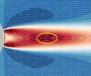
Figure 7. Mean streamlines for different values of  $\beta$. Background colour plots indicate the streamwise component
  $u$ (parallel to
  $U_\infty$) with blue and red positive and negative values, respectively; white arrows indicate the streamlines and yellow lines emphasise those bounding the recirculation bubbles.
  $Re=25\,000$. Results are shown for (a)
  $\beta =0$, (b)
  $\beta =0.12$, (c)
  $\beta =0.16$, (d)
  $\beta =0.21$, (e)
  $\beta =0.28$, ( f)
  $\beta =0.33$.
It is classically argued (e.g. Bearman Reference Bearman1967; Leal & Acrivos Reference Leal and Acrivos1969) that a recirculating bubble is formed when the entrainment needs of the two separated shear layers can only be met by some extra fluid that has to be provided from further downstream – hence, the necessary ‘closure’ of the two separating mean streamlines, with some of the fluid between the two shear layers thus having negative mean axial velocity, having been injected from around the rear stagnation point. When there is sufficient bleed fluid through the porous plate to provide the shear layers’ entrainment needs, there is no need for further fluid to be added to the near wake (from further downstream) so that a recirculating region does not form. It seems likely that at that stage the shear layers are sufficiently diffuse to prevent the usual interaction between them leading to Kármán shedding. But it is not really clear if such shedding can still occur without the bubble or, indeed, whether shedding always occurs if there is a bubble. More recent analyses, like that of Steiros et al. (Reference Steiros, Bempedelis and Ding2021), generally assume the flow is steady, so make no direct link between the existence of a bubble and the Kármán shedding process. In fact, there must be a specific porosity marking the boundary between bubble and no-bubble appearance, whereas such a firm boundary between shedding and no-shedding seems less likely. It is therefore important to study the major unsteady features of the wake in more detail and this is addressed in § 3.2.
First, however, given that it is well known that the energy in the fluctuating motions in the wake (particularly the cross-stream component) is largest in the region of the vortex formation – around the mean streamline closure marking the end of the bubble – we show in figure 8 the flow fluctuations on the wake centreline ( $y=0$). These data are derived from the PIV measurements. Figures 8(a) to 8(e) show the spectra of the fluctuating velocity (
 $v'$) along the
  $x$ direction for different values of
  $\beta$, whilst figure 8( f) shows the fluctuating energy level, measured as
  $(\overline {u'^2} + \overline {v'^2})/U_\infty ^2$, in the region up to about
  $x/D=20$. A dominant frequency is clear in most cases, with
  $fD/U_\infty \approx 0.15$, although close inspection shows that this Strouhal number is not fixed but decreases a little with increasing
  $\beta$, consistent with figure 5(b). Note that the first appearance of a clear peak in the spectrum occurs at increasing
  $x/D$ as
  $\beta$ increases; even at
  $\beta =0.12$ a peak does not appear until around
  $x/D=1.0$. This seems consistent with the fact that peaks in drag spectra do not appear once
  $\beta \ge 0.12$, for the possible reasons discussed above – i.e. the shedding is not initiated until further downstream once
  $\beta >0$ and the flows through the holes in the plate might be expected to influence the fluctuating pressure field.

Figure 8. (a–e) Spectra of the  $v'$ component along the centreline (
 $y/D=0$). The colour bar for the spectral plots indicates PSD levels with an arbitrary scale, running from the highest (red) to the lowest (yellow/white) level, for which the frequency resolution is
  $\Delta f D/U_\infty \approx 0.007$. ( f) Fluctuation energy along the centreline; solid circles indicate the
  $x/D$ location of the downstream end of the bubble, if it exists – see figure 7 – and, likewise, these locations are shown by the vertical dashed lines in (a–e). All data are from the PIV measurements. Results are shown for (a)
  $\beta =0.12$, (b)
  $\beta =0.16$, (c)
  $\beta =0.21$, (d)
  $\beta =0.28$, (e)
  $\beta =0.33$. ( f) Fluctuating energy on
  $y=0$.
Roshko (Reference Roshko1954) proposed a universal Strouhal number based on the maximum distance between the separated shear layers (i.e. the wake width,  $H$) and the velocity just outside the shear layers at the separation points. The latter is related to the difference between the free-stream velocity and the centreline values near the plate and clearly decreases with increasing
  $\beta$. The wake width is related to the thickness of the shear layers (the ‘diffusion’ length, as argued by Gerrard Reference Gerrard1966). Figure 7 shows that this wake width
  $H$ also decreases with
  $\beta$, so for a constant value for the universal Strouhal number (about 0.16 according to Roshko Reference Roshko1954), only small changes in shedding frequency
  $f_s$ might be expected – again consistent with the present data. The frequency signature for
  $\beta =0.33$ suggests a much broader spectral peak, making it difficult to identify any particular peak, as discussed earlier in the context of the hot-wire data.
The centreline energy levels shown in figure 8( f) have, at least for the lower values of  $\beta$, a clear peak around the location of the end of the bubble in each case (cf. figure 7), consistent with that being the region of vortex formation, as observed for solid bluff bodies (Szepessy & Bearman Reference Szepessy and Bearman1992). There is a relatively rapid fall in peak energy, particularly beyond
  $\beta \approx 0.16$, with more than an order of magnitude difference in the peak values at
  $\beta =0$ and 0.33. Based on these data one might speculate that Kármán shedding ceases beyond about
  $\beta =0.2$ but, again, details of any transition region are unclear so, in the next section, we explore this further by using coherence and phase measurement within the wake.
3.2. Using coherence data to diagnose vortex shedding
When regular vortex shedding occurs, a measurement of the coherence in the axial velocity between two locations on opposite sides of the wake will yield near-unity coherence with a  $180^\circ$ phase difference at the shedding frequency (because vortices are shed alternately from each side). In the laminar flow regime (with a Reynolds number of, say, around 100) the vortex street continues regularly all the way downstream from its inception; there must then also be a perfect coherence at twice the shedding frequency, but with zero phase difference. Only the action of diffusion will eventually weaken the coherence at the higher harmonics. In the present case of high Reynolds number, for which the flows are always fully turbulent, these higher harmonic coherence peaks might be expected to weaken considerably. Even at the shedding frequency, there will not be perfect coherence because the background turbulence inevitably broadens the spectrum somewhat – there is ‘jitter’ in the signals.
Two hot-wire probes were used for the present measurements, each placed around the centre of the two shear layers at the same distance downstream, as shown in figure 9. The data presented below were obtained for an averaging period of 240 s (typically equivalent, at  $Re=26\,000$, to some 3200 shedding cycles in cases where Kármán shedding occurred), with the probes located at
  $x/D=6.2$ and
  $y/D=\pm 0.8$. It was found that changes in these locations had little effect on the resulting data.

Figure 9. Position of the probes for the wind tunnel experiments with respect to the recirculation bubbles for several values of  $\beta$. Black dots at
  $x/D=6.2$ show the probe locations. The recirculation bubbles are indicated by the bounding mean streamlines, as identified from the PIV data shown in figure 7.
We denote the coherence by  $C_{u_1u_2}$ and the corresponding phase by
  $\phi$, determined in the usual way from the cross-spectra between the two signals
  $u'_1$ and
  $u'_2$. The plots in figure 10 show the results for four plates in the range
  $0.1\le \beta \le 0.33$. Coherence values close to unity indicate a high level of synchronisation whereas lower values indicate weaker synchronisation. For
  $\beta =0.1$ and 0.19, there is strong coherence at
  $f_sD/U_\infty \approx 0.14$, with a phase shift of
  $\phi \approx 180^\circ$, indicating that the two signals are closely in anti-phase, consistent with classical vortex shedding. For
  $\beta =0.24$, a similar peak appears at about the same frequency, with similar values of
  $\phi$, also consistent with vortex shedding, but there is no sign of a second peak at the frequency of the first harmonic. A second peak, the first harmonic, does occur for
  $\beta =0.1$ and
  $\beta =0.19$ with a phase shift close to
  $0^\circ$, indicating the two signals are in-phase at this frequency, as expected. In both these cases there is also a hint of the second harmonic, at three times the shedding frequency. For all the other frequencies, the coherence value is near zero and the phase shift shows scattered values, indicating a lack of coherence, caused entirely by the turbulence fluctuations at each location. For
  $\beta =0.33$, figure 10(d), there is no sign of any peak.

Figure 10. Coherence between two velocity signals at each shear layer ( $C_{u_1u_2}$) and its phase shift (
 $\phi$) for four different porosity levels
  $\beta$.
  $Re=65\,000$. Results are shown for (a)
  $\beta =0.10$, (b)
  $\beta =0.19$, (c)
  $\beta =0.24$, (d)
  $\beta =0.33$.
To provide further insight, we have evaluated spectral proper orthogonal decompositions (SPODs) from the PIV fields acquired in the second field of view (FoV) (figure 4b), from  $5.5< x/D<13$. Details about SPOD and the algorithm used can be found in Towne, Schmidt & Colonius (Reference Towne, Schmidt and Colonius2018). Each data set had 3000 fields, comprising a time scale equivalent to at least 200 periods of vortex shedding. Eight SPOD modes have been computed for each plate. Figures 11(a) and 11(c) show the SPOD energy levels of each mode versus frequency for two cases,
  $\beta =0.16$ and 0.21. Only the first four modes are shown because the energy contents of the other four are negligible. In both cases the first mode is more energetic and contains the only peaks observable. Interestingly, the energy level plots for the first mode have similarities to the coherence plots, suggesting that they are related to the same physical mechanism in the flow. The first peak is clearly associated with vortex shedding, as the mode shapes in figures 11(b) and 11(d) illustrate. The pair of lobes with alternate velocity fluctuation levels are consistent with the pair of vortices of a typical von Kármán street and are also consistent with the phase shift
  $\phi \approx 180^\circ$ found at the first peak in figure 10. As for the second peak, the shapes reveal that it constitutes a harmonic of the vortex shedding. The signal of the velocity fluctuations at
  $y/D=\pm 0.8$ are in-phase, explaining the phase shift of
  $\phi \approx 0^\circ$ observed for the second peak.

Figure 11. Spectral POD at  $Re=35\,000$ for (a,b)
  $\beta = 0.16$ and (c,d)
  $\beta = 0.21$. The mode shapes in (b,d) correspond to the frequencies identified and marked with symbols in (a,c).
The key question is to understand why the second peak appears only if  $\beta$ is small enough. We noted above that this second peak can only appear if vortex shedding is sufficiently regular (by which we mean, continuous in time). If, for whatever reason, the vortex shedding process is intermittent and, thus, does not continue for long enough periods of time, then the first peak will be weaker and the second peak (the harmonic) is rather less likely to appear – it may simply become submerged in the background spectral energy. Figure 12 shows examples of typical instantaneous axial velocity and spanwise vorticity fields for three cases, taken from the PIV data. Figure 12(a,d) (
 $\beta =0.12$) shows a pattern indicative of periodic vortex shedding and typical of a process yielding a coherence plot with two peaks. In figure 12(b,e) (
 $\beta =0.26$) the patterns show evidence of some shear layer interactions but without evidence of the usual shedding structure at that particular time. The coherence plot for this case, however, shows one peak, suggesting that shedding does occur from time to time; figure 10(c) shows the coherence for a case with a very similar
  $\beta$. Figure 12(c, f) (
 $\beta =0.33$) shows a case completely devoid of shedding, so that the coherence plot has no peaks at all – recall figure 10(d) for a coherence plot of a closely similar case.

Figure 12. Three instantaneous fields of the total mean velocity (a–c) and vorticity  $\omega$ (d–f), characteristic of the three states observed for
  $0\leq \beta \leq 0.35$: (a,d) regular and periodic vortex shedding, (b,e) irregular vortex shedding and (c, f) no vortex shedding. Results are shown for (a,d)
  $\beta =0.12$, (b,e)
  $\beta =0.26$, (c, f)
  $\beta =0.33$.
3.3. Results for all plates
Data like those in figure 10 were used to compile coherence maps over the whole range of  $\beta$. These are shown in figure 13 for
  $Re=38\,000$. The first peak at
  $fD/U_\infty \approx 0.14$ forms a clear signature that ranges all the way from
  $\beta =0$ to a little less than
  $0.3$. The second peak, associated with vortex shedding that is fairly regular throughout the whole measurement period, also has a well-defined signature ranging from
  $\beta =0$ to
  ${\approx }0.2$ but there is no second peak beyond that and, as noted above, the main peak at the shedding frequency also disappears beyond
  $\beta \approx 0.28$. One can thus tentatively divide the
  $\beta$ range into three regions, as shown in the figure, with the central region having only the major shedding peak present. The start of this region is around
  $\beta =0.22$, which is roughly where Castro (Reference Castro1971) deemed vortex shedding to ‘switch off’. On the other hand, Steiros et al. (Reference Steiros, Bempedelis and Ding2021) suggested that vortex shedding ceases around
  $\beta =0.3$. How can these various observations be reconciled?

Figure 13. Coherence (a) and phase (b) for the porous plates with varying porosity  $\beta$ at
  $Re=38\,000$. Data for all
  $\beta$ values between those available (indicated by the red diamonds) were simply interpolated to provide smooth variations.
Now recall that the coherence plots shown thus far were computed using the long-time series of  $T=240$ s. They therefore only show the long-time-average state, but do not directly address the degree of intermittency in the shedding. To obtain more information about the wake behaviour through time, the total time period was divided into consecutive sub-intervals (
 $\Delta T$) of either twelve or 1.2 s. Each of these was thus either 5 % or 0.5 % of the total available sample period,
  $T$, representing typically 300 or 30 shedding cycles, respectively. Here
  $C_{u_1u_2}$ and the corresponding phase
  $|\phi |$ were computed for each sub-interval. Figure 14 shows the coherence and phase data for the particular case of
  $\beta =0.12$ and for both values of
  $\Delta T/T$. All the coherence values in this figure have been normalised by their long-time-average coherence values in their particular frequency band; so
  $C_1^*$ is the coherence normalised by the maximum long-time average (closely 1.0) of
  $C_{u_1u_2}$ within the frequency band
  $0.12\le fd/U_\infty \le 0.16$ and
  $C_2^*$ is the coherence normalised by the maximum long-time average (0.75) of
  $C_{u_1u_2}$ within the frequency band
  $0.26\le fd/U_\infty \le 0.32$.

Figure 14. Plots (a,b) show the maximum value of  $C_{u_1u_2}$ within the two frequency ranges
  $0.12\le fd/U_\infty \le 0.16$ (blue symbols) and
  $0.26\le fd/U_\infty \le 0.32$ (red symbols), as a function of time through the entire record. Results are shown for (a,c,e)
  $\Delta T/T=0.005$ and (b,d, f)
  $\Delta T/T=0.5$. The lower plots show the normalised coherences
  $C_1^*$ and
  $C_2^*$ (c,d) and corresponding
  $|\phi |(f)$ (e, f) within each
  $\Delta T$ sub-interval, with their values indicated by the contour scale.
  $\beta =0.12$,
  $Re=26\,000$.
The top plot in each case shows the maximum coherence value that occurs within those two frequency bands. Not surprisingly, there is significantly higher scatter in the data when  $\Delta T$ is only
  $0.005T$, figure 14(a,c,e), but the presence of the second (higher frequency) peak is evident throughout practically the whole time period provided
  $\Delta T$ is large enough; see figure 14(b,d, f). If it is very short – as in figure 14(a,c,e) – there are many periods within which, although the maximum secondary peak value may be quite large, the average over that period is very small – compare the red symbol data in the top two plots of figure 14(a,c,e). Such periods correspond to normalised
  $C_{u_1u_2}$ values for the first peak being much lower than average – typically around 0.7, although it is difficult to identify those specific
  $\Delta T$ periods within figure 14(a,c,e). Note too that, for
  $\Delta T/T=0.005$, there is considerable variability in the frequency at which the first peak appears; see the
  $C_1^*$ data in figure 14(a,c,e). This is a result of the influence of the background turbulence field, which leads to significant ‘jitter’ in the shedding frequency, and is the main reason why we chose to use the two frequency bands rather than specific frequencies. This jitter effect is reduced markedly when longer
  $\Delta T$ periods are used, as is clear in figure 14(b,d, f). Only very occasionally are there then periods during which the secondary peak is (on average) hardly apparent; data for times between
  $t/T=0.6$ and 0.7, in particular, suggest the lack of a secondary peak on average, consistent with a significant reduction in the maximum
  $C_2^*$ value (see the top plot). Data presented from now on will be those obtained with the longer sub-interval of twelve seconds, on the basis that this is a long enough averaging period to minimise the effect of this turbulence-induced jitter in the observed shedding process. Note, incidentally, that alternative values of
  $\Delta T/T$, intermediate between those used for figure 14, were tried but the results added nothing to the physical interpretations of the data.
We may define the vortex shedding intermittency,  $I_{VS1}$, as the proportion of those sub-intervals that contain a first correlation peak within a frequency range of
  $0.12\le fd/U_\infty \le 0.16$ and having a
  $C_{u_1u_2}$ of at least 0.6 – i.e.
  $\sum _{i=1}^{i_{last}}i/I$, where
  $i=1$ and
  $i=i_{last}$ denote the first and last sub-periods having such a peak, and
  $I$ is the total number of sub-periods (20 for
  $\Delta T/T=0.05$). Equivalently, the intermittency is the time sum of those short periods containing that first peak divided by the total time period,
  $\sum \Delta T_{peak}/T$. A similar calculation was performed for the appearance of a second correlation peak within the frequency range of
  $0.26\le fd/U_\infty \le 0.32$ (i.e. the first harmonic of the vortex shedding frequency), having
  $C_{u_1u_2}=0.6$ at least. This is denoted by
  $I_{VS2}$. Figure 15 shows the intermittency for both peaks (including values obtained with a less demanding cutoff value of 0.4 for the coherence), along with the time variation of coherence values,
  $C_1^*$ and
  $C_2^*$, within the two frequency ranges (
 $0.12\le fd/U_\infty \le 0.16$ and
  $0.26\le fd/U_\infty \le 0.32$), and their corresponding phases, all as a function of porosity.

Figure 15. Shedding intermittency (a,b), normalised coherence values,  $C^*$, (c,d) and phase,
  $\phi ^*$, (e, f) over all
  $\beta$, for the frequency ranges (a,c,e)
  $0.12\le fd/U_\infty \le 0.16$ (i.e. for the first peak) and (b,d, f)
  $0.26\le fd/U_\infty \le 0.32$ (i.e. the second peak). Note that each horizontal bar appearing in the lower plots refers to the corresponding
  $\beta$ value above it in the top plots.
It is immediately clear that up to  $\beta$ of around 0.26, the first peak coherence is uniformly high across all the sub-intervals (i.e. throughout all the total period
  $T$), but it falls rapidly for greater
  $\beta$. Up to a rather lower
  $\beta$, around 0.22, the second peak's coherence value is also quite high, rarely dropping below about 0.4. The intermittency of this second peak begins to fall fairly rapidly beyond about
  $\beta =0.22$, consistent with the earlier tentative supposition that this marks the beginning of a transition range, within which the time consistency of the vortex shedding begins to get weaker, evidenced first by a less consistent appearance of the second peak. The precise point at which the intermittencies begin to fall clearly depends somewhat on the cutoff values used (0.4 or 0.6 in the figure), but it is clear that the second peak decaying earlier than the first is independent of the criteria used. Note that within and beyond the transition range the
  $\Delta T$ periods that exhibit high coherence peaks for either the first or the second peak are randomly distributed in time. There is thus no longer a time scale governing when the shedding ‘switches’ on and off during the full time period,
  $T$. Note also that, for values of
  $\beta$ in excess of about 0.3 (around the end of the transition range), the intermittency of the second peak can exceed that of the first. We return to this point in § 3.4.
We conclude that the transition region between  $\beta \approx 0.22$ and 0.3, shown in figures 13 and 15, is characterised not by a sudden ‘switching off’ of the shedding process but by a fairly rapid reduction in the period of time over which the second peak appears, from
  $\beta \approx 0.22$ onwards, followed by a similarly rapid reduction in the total period of time over which the major shedding peak occurs, beyond
  $\beta =0.26$. Kármán shedding does not simply cease entirely beyond
  $\beta =0.22$, although it then lacks sufficient energy when averaged over all time to yield significant energy at the first harmonic. It is interesting that the recirculating bubble is not present beyond about
  $\beta =0.28$, see figure 9, which is when one can conclude from figure 15 that Kármán shedding hardly exists, except perhaps for occasional, very short periods of time.
It might be asked whether the particular arrangement of the holes in the plate affects the global wake behaviour. In the early Castro (Reference Castro1971) experiments, the holes, of diameter  $d$, were arranged in a staggered pattern of three rows, with a range of
  $\beta$ provided by
  $0.077< d/D<0.308$. Reynolds numbers based on hole size thus varied from about 1300 to 5200 when
  $Re=UD/\nu \approx 17\,000$ (the value used to elucidate the behaviour of the separated bubble). The present experiments used four rows of aligned, octagonal holes (see figure 3), covering the range
  $0.046< d/D<0.08$, with a corresponding Reynolds number range of
  $1150< Re_d<2000$ when
  $Re=25\,000$ (the value used for the data shown in figure 7). Despite these differences, which amounted to a factor of two difference in
  $Re_d$ for any given
  $\beta$, we have seen that the two sets of experiments yield an overall behaviour of the wake as
  $\beta$ varies that is very similar. In particular, the variation of quantities like
  $C_d$ and
  $St$ with Reynolds number is practically the same and the way in which the separated region moves downstream and changes size and shape as
  $\beta$ increases is the same. For example, the mean flow bubble has in both cases disappeared by
  $\beta =0.33$ but is still present for
  $\beta =0.28$. Very close to the plate there must naturally be significant differences in the detailed flow, but it seems that the relatively very small-scale motions, particular to the jet flows through the holes and the wakes behind the solid pieces between them, are rapidly assimilated into the much larger-scale motions in and downstream of the separated bubble without having any lasting influence.
3.4. The steady wake at large  $\beta$

Given that once  $\beta$ exceeds around 0.28 no Kármán vortex shedding appears, it is pertinent to consider to what extent the wake resembles classical self-similar wakes far downstream of two-dimensional bluff bodies. We therefore present some wake data for the
  $\beta =0.33$ case, deduced from the PIV data that covers the wake region up to
  $x/D\approx 20$. Figure 16 shows cross-stream axial velocity and turbulence energy profiles, normalised in the standard way using
  $u_o$, the difference between the free-stream velocity (
 $U_\infty$) and the velocity on the wake centreline, and
  $L$, the width of the wake measured as (one half of) the distance between the points where the velocity difference is one half of its maximum. Self-similarity for a two-dimensional wake requires that
 \begin{equation} \frac{U_\infty^2}{u_o^2}=A\left(\frac{x-x_o}{2D}\right) \quad\textrm{and} \quad \frac{L^2}{D^2}=B\left(\frac{x-x_o}{2D}\right), \end{equation}
where  $A$ and
  $B$ are constants. It is well known that even a long way downstream of the wake generating body, although similarity in this form usually exists, there is wide variation in what ideally would be universal parameters. For example, the wake spreading rate,
  $\alpha =({U_\infty }/{u_o})({{\rm d}L}/{{\rm d}\kern0.7pt x})$, can vary widely depending on the body shape – initial conditions are not ‘lost’, at least at the distances that can normally be covered in experiments or computations. In the present case one would not really expect good similarity in the relatively short and early part of the wake that our experiments covered. Nonetheless, estimating
  $L/D$ and
  $u_o/U_\infty$ from the raw profiles led to reasonable collapse of the normalised axial velocity profiles, as seen in figure 16(a). The spreading rate can be expressed as
  $\sqrt {AB}/4$ that, using data from the best fit line to
  $L^2/D^2$ vs
  $x/D$, figure 16(c), leads to
  $\alpha =0.173$. This is very different to that found by Wygnanski, Champagne & Marasli (Reference Wygnanski, Champagne and Marasli1986) in their experiments on the wake of a 70 % solidity plate (i.e.
  $\beta =0.3$), which had
  $\alpha =0.09$. This difference is not surprising because their measurements were obtained (roughly) over the range
  $400<(x-x_o)/D<1600$. The very much higher turbulence intensities in the near wake must inevitably lead to a more rapid growth of the wake initially. Whilst reasonable local similarity is evident in the velocity profiles in our near-wake region, the normalised axial turbulence energy profiles, figure 16(b), are far from collapse although there is a clear trend towards such collapse as
  $x/D$ increases. Indeed, the centreline value of
  $u'^2/u_o^2$ at
  $x/D=19.5$ is not very far below the value found by Wygnanski et al. (Reference Wygnanski, Champagne and Marasli1986). Incidentally, their
  $\alpha$ for a solid flat plate was 0.072 compared with 0.09 for the 70 % solidity plate, illustrating the lack of universal behaviour in these wakes even at such long distances downstream. It is interesting that they concluded that the wake behind the solid plate (which no doubt shed a Kármán vortex street) reached a self-preserving state more rapidly than the wake behind the porous plate.

Figure 16. (a) Transverse profiles of the axial velocity for  $\beta =0.33$. (b) Corresponding profiles of the axial turbulence energy. The legends show values of
  $x'=x/D$. (c) Growth of the wake. (d) Variation of the centreline axial energy. The solid red symbols in (c,d) are for
  $\beta =0.15$, Note that slightly different values of
  $x_o$ have been used in (c,d).
Note that figures 16(c) and 16(d) include data obtained for a much lower porosity case,  $\beta =0.15$. This is well within the vortex shedding regime and although, curiously perhaps, the mean velocity profiles at the four
  $x'$ locations (not shown) do happen to collapse when normalised using the
  $L/D$ and
  $u_o/U_\infty$ values appropriate for each, these values show clearly that this close to the plate even the mean flow is very far from any hint of local similarity. Importantly for the present context, Wygnanski et al. (Reference Wygnanski, Champagne and Marasli1986) also identified large-scale structures in their wakes. In particular, in the wake of a
  $\beta =0.7$ plate, they found that the predominant frequency at the most upstream location –
  $(x-x_o)/D\approx 10$ – was around
  $fD/U_r=0.3$. A very similar result was obtained by Cimbala, Nagib & Roshko (Reference Cimbala, Nagib and Roshko1988) at
  $x/D=10$ in the wake of a
  $\beta =0.47$ flat plate. This is about double the vortex shedding frequency of a solid plate, which suggests that the natural instability in the wake profile at that point downstream is actually not far from twice the vortex shedding frequency, whether or not such shedding actually occurs – so it is not in fact a ‘second harmonic’ at all. This may help to explain why, for
  $\beta >0.3$, the coherence peak at what seems to be the second harmonic can still appear and, indeed, appear more frequently than the first peak, as noted earlier. Recall also that figure 12(c, f) (for
  $\beta =0.33$) indicates the presence of large-scale structures, although these have not yet developed into the form typically seen in far wakes by, for example, Wygnanski et al. (Reference Wygnanski, Champagne and Marasli1986).
A related explanation for the broad coherence peak (when  $\beta >0.3$) at a frequency significantly larger than the low-
 $\beta$ vortex shedding frequency is provided by the work of Huang & Keffer (Reference Huang and Keffer1996). They explored the wake in the range
  $1< x/D<20$ behind a two-dimensional mesh with
  $\beta =0.4$. By studying spectra of the transverse velocity (
 $v'$) and coherence from autospectra of two such signals obtained on either side of the wake, they showed that the small-scale structures that develop in the two initially independent shear layers merge to form quasi-periodic larger structures further downstream, having a characteristic frequency equivalent to
  $St\approx 0.19$. This began to be evident as early as
  $x/D=5$. It seems likely that the large-scale structures Huang & Keffer (Reference Huang and Keffer1996) identified are precisely those found by Wygnanski et al. (Reference Wygnanski, Champagne and Marasli1986), as indeed the former authors recognised. In any case, they are very different from the Kármán-type vortex structures that appear at lower porosities.
4. Final discussion and conclusions
This paper has focused on the characterisation of the vortex shedding pattern in the flow past flat porous plates in the range  $0 \leq \beta \leq 0.35$ based on a series of experiments carried out at Reynolds numbers between 15 000 and 70 000. The main objective was to understand how the flow evolves from the regular von Kármán street, typical of two-dimensional bluff bodies, to a wake without any vortex shedding. It has been shown that the subtleties in vortex shedding cannot be fully identified from drag force measurements on the plate or, indeed, from a single probe in the near wake. We have used coherence and phase data from twin probes to identify some of these subtleties.
The general behaviour of the wake – i.e. a fall in the plate's drag coefficient and Strouhal number as porosity increases – is in line with the conclusions of earlier works. However, three distinct wake patterns have been characterised and are illustrated in figure 12. The first is the classical von Kármán vortex street, with regular and periodic shedding of vortices having a well-defined frequency. This is characterised by two peaks in the coherence spectrum, associated with the frequency of vortex shedding and its first harmonic. Spectral peaks at higher harmonics are largely absent because of the diffusion-like effects of the high-intensity turbulence in which the vortex street exists. The second pattern represents an irregular vortex shedding process, in which the Kármán shedding occurs for short periods, interspersed randomly with periods when it ceases. This process was identified by sub-dividing the total sampling length into shorter intervals, which allowed definition of a shedding intermittency – the proportion of total time during which shedding occurred, giving the fundamental spectral peak at the Strouhal frequency. As the porosity increases through this second range of  $\beta$, this intermittency decreases, in the sense that the shedding periods become shorter and less frequent, with concomitant reduction in the energy at the shedding frequency and a fairly rapid disappearance of the second peak. The third pattern is characterised by almost no periods of vortex shedding, so that the shedding intermittency is very small. On average, the vortex shedding pattern is dominant for the cases having
  $\beta \leq 0.22$, whereas the non-vortex shedding pattern occurs once
  $\beta$ exceeds about 0.28. Between these two (necessarily approximate) limits, the wake is in the transition regime, with irregular vortex shedding sufficient to give a clear spectral peak at the fundamental frequency but (increasingly) none at the first harmonic.
A natural question concerns why, in the transition regime, the vortex shedding only lasts for relatively short periods and then apparently disappears, before reappearing later. The very early stability analysis of von Kármán, mentioned in § 1, indicated that a street composed of a staggered array of idealised point vortices was stable to first-order two-dimensional disturbances provided the ratio ( $a/b$) of lateral to longitudinal spacing between them was 0.281. However, it was subsequently shown that this system is in fact unstable at the second order of approximation in the disturbance amplitude (Kochin Reference Kochin1939) but, more importantly, that the stability could be critically affected if the vortices are of finite size (and could change shape); see, for example, Saffman & Schatzman (Reference Saffman and Schatzman1982) and Maches et al. (Reference Maches, Bartley, Borjon and Carretero-González2021). Such analyses were all in the context of an irrotational, uniform velocity free stream. In practical cases like those studied here, the vortices are certainly of finite size right from their inception and they are also embedded in a highly turbulent and sheared flow. Nonetheless, although it undoubtedly takes some axial distance before the regular vortex street develops into its final stable state for low-
 $\beta$ cases, and probably much further downstream than where our PIV data were gathered, typical vortex spacings from the present PIV measurements in the early wake are not inconsistent with the classical Kármán result of
  $a/b=0.28$. However, it is not at all surprising that for larger
  $\beta$ (in the transition regime), even during the sub-periods when shedding occurs, the vortex pattern seems to be quite different, so that those ‘segments’ of vortex street have an unstable configuration. The street therefore cannot last for long because of the very significant (three- as well as two-dimensional) disturbances. With increasing amounts of bleed air and the subsequent further movement downstream of the separated region, it is increasingly unlikely that the much weaker and more diffuse vortices resulting from the roll-up of the two shear layers can sustain any stable configuration. Eventually, as we have seen, they do not form at all.
We suggested in § 3.3 that the particular arrangement of the holes in the plate has little effect on the overall, large-scale behaviour of the wake. It is interesting that the same conclusion was reached by Perera (Reference Perera1981) in their study of porous plates mounted on a wall; they found no effect of the type of porosity on the large-scale behaviour. They also found, incidentally, that the mean flow bubble disappeared once  $\beta$ exceeded about 0.3, in line with the present results. On the other hand, in tests over a wall-mounted fence with
  $\beta \approx 0.38$, Kim & Lee (Reference Kim and Lee2001) found a distinct effect of hole arrangement (varying size and spacing but with constant
  $\beta$). This is perhaps not surprising, since at such a high porosity the ‘life time’ of the individual, smaller-scale structures downstream of the holes will inevitably be greater, since they are not rapidly engulfed by the highly turbulent, often reversing flow that exists near the plate at low
  $\beta$. It is also worth noting that in the recent direct numerical simulation study of Singh & Narasimhamurthy (Reference Singh and Narasimhamurthy2022) on porous plates, which explored the nature of the flow very near the plate, the authors found that the plate's perforations led to a transitional state in the near wake. However, their
  $Re$ (
 $U_\infty D/\nu$) was only 250, so the jet flows through the holes were laminar and detailed comparisons with the present data are perhaps inappropriate. Nonetheless, they observed that the drag coefficient and Strouhal number variations with
  $\beta$ had ‘excellent qualitative agreement with the high Re experiments of Castro (Reference Castro1971)’.
In the cases when virtually no vortex shedding occurs, the wake displays some local similarity but, not surprisingly, this is far from complete (there is no self-similarity in the turbulence profiles); it is non-existent when regular Kármán shedding occurs. The remaining hints of a coherence or spectral peak at a significantly higher frequency (perhaps in the range  $0.2< St<0.3$) may, in fact, be evidence more of the natural wake instability found by other authors or of the large-scale structures resulting from the merging of smaller structures in the very near wake, rather than any very occasional periods of Kármán vortex shedding.
Within the  $Re$ range covered, the results presented here are only weakly dependent on
  $Re$, suggesting a universal behaviour of the wake response to varying porosity since the minimum
  $Re$ number (in excess of 20 000) was sufficient to yield a fully turbulent wake. It seems likely that two-dimensional porous bodies of any shape would display the same three regimes as porosity increases: Kármán shedding at low porosity, no shedding at high enough porosity and a transition regime between them, in which shedding becomes increasingly irregular. We do not speculate about the wake behaviour behind porous two-dimensional axisymmetric bodies (like discs or spheres), not least because of the rather different vortex shedding processes in such cases. This would be an interesting topic for further study.
Funding
We gratefully acknowledge the financial support from EPSRC (grant no. EP/S013296/1) and the various helpful comments of the reviewers. Pertinent data for this paper are available at doi: https://doi.org/10.5258/SOTON/D3022.
Declaration of interests
The authors report no conflict of interest.


 Open access