
Water-Level Prediction Analysis for the Three Gorges Reservoir Area Based on a Hybrid Model of LSTM and Its Variants
1
Institute of Disaster Prevention, Sanhe 065201, China
2
Hebei Key Laboratory of Resource and Environmental Disaster Mechanism and Risk Monitoring, Sanhe 065201, China
*
Author to whom correspondence should be addressed.
Water 2024, 16(9), 1227; https://doi.org/10.3390/w16091227
Submission received: 22 March 2024
/
Revised: 19 April 2024
/
Accepted: 23 April 2024
/
Published: 25 April 2024
Abstract
:The Three Gorges Hydropower Station, the largest in the world, plays a pivotal role in hydroelectric power generation, flood control, navigation, and ecological conservation. The water level of the Three Gorges Reservoir has a direct impact on these aspects. Accurate prediction of the reservoir’s water level, especially in the dam area, is of utmost importance for downstream regions’ safety and economic development. This study investigates the application and performance of four distinct deep-learning models in predicting water levels. The models evaluated include the Long Short-Term Memory (LSTM), Bidirectional Long Short-Term Memory (BiLSTM), Convolutional Neural Network–Long Short-Term Memory (CNN–LSTM), and Convolutional Neural Network–Attention–Long Short-Term Memory (CNN–Attention–LSTM). The performance of these models was assessed using several metrics, namely the Coefficient of Determination (R2), Mean Absolute Error (MAE), Root Mean Squared Error (RMSE), and Mean Absolute Percentage Error (MAPE). The findings indicate that the CNN–Attention–LSTM model outperforms the others in all metrics, achieving an R2 value of 0.9940, MAE of 0.5296, RMSE of 0.6748, and MAPE of 0.0032. Moreover, the CNN–LSTM model exhibited exceptional predictive accuracy for lower water levels. These results underscore the potential of deep-learning models in water-level forecasting, particularly highlighting the efficacy of attention mechanisms in enhancing predictive accuracy. Precise water-level predictions are instrumental in optimizing hydropower generation and providing a scientific basis for effective flood control and water resource management.
1. Introduction
Water resources are essential for maintaining an ecological balance and sustainable economic development. As one of the most significant hydropower projects in the world, the Three Gorges Hydropower Station and its reservoir play a crucial role in agriculture, industrial development, and human survival in the Yangtze River Basin [1]. The Three Gorges Reservoir, as the core of water resource management in this basin, plays a significant role in flood control, water supply, irrigation, and hydropower generation by regulating the overall river flow. It also plays a crucial role in regional climate regulation and ecological conservation. Therefore, accurate prediction of the reservoir’s water level is essential for reservoir management, ensuring safe operation, rational allocation of water resources during dry seasons, and managing reservoir storage during flood seasons to ensure the safety of downstream areas [2].
In the current context of water resource management and flood prevention, an accurate water-level prediction is crucial for planning and emergency responses. The development of machine-learning techniques offers the potential for more precise water-level predictions. With the rapid development of machine-learning technology, significant progress has been made in its application to water-level predictions. This paper provides a comprehensive review of fundamental research in this field, focusing on data preprocessing techniques, ensemble learning methods, and the contribution of deep-learning models to improving the accuracy of water-level predictions.
Data preprocessing is a key step in building efficient models and can significantly enhance the accuracy of predictions. The study by Wu et al. [3] highlighted the importance of data preprocessing in river water-level predictions, where data cleaning and transformation effectively improved model performance. The work of Huang et al. [4] and Lee and Ouarda [5] further confirmed the utility of data preprocessing in enhancing the performance of hydrological models. A comparative study of three hydrodynamic models for Lake Ontario by A. N. Huang et al. [6] applied to water quality and quantity management of large lakes, environmental engineering, and ecological restoration projects. M. Vahid et al. [7] compared the efficacy of autoregressive moving average and integrated moving average models in inflow predictions. Zhu et al. [8] and Wang et al. [9] demonstrated new advances in signal denoising and feature extraction by introducing Empirical Mode Decomposition (EMD) and Variational Mode Decomposition (VMD) techniques, which are particularly important for dealing with nonlinear and non-stationary hydrological time series data. Through data preprocessing techniques combined with traditional methods (such as empirical and formulaic approaches), simple prediction tasks can be conducted. However, given the complexity and nonlinearity of the data, the limitations of these methods in terms of prediction accuracy become particularly evident. With the development and application of machine-learning technology, which is capable of handling complex data patterns, new avenues are provided to overcome these traditional limitations.
Ensemble machine-learning methods, which combine multiple models to improve the accuracy and robustness of predictions, have been widely applied in hydrological forecasting. Bagging, proposed by Breiman [10], and Boosting, proposed by Friedman [11,12], are two pillars of ensemble learning, reducing model bias and variance through different strategies. M. Vahid used ANN and ARIMA models to predict the Caspian Sea level [13], which is significant for environmental monitoring and planning in coastal areas and for developing strategies to cope with sea-level rises. G. Y. Xu et al. [14] developed a water-level-prediction model based on ARIMA-RNN, applicable for water-level management and prediction in rivers and reservoirs and disaster warning systems. In hydrology, the studies by Anctil and Lauzon [15], as well as Snelder et al. [16], demonstrated the effectiveness of these ensemble methods in improving the accuracy of water-level predictions. F. Mekanik et al. [17] used multiple regression and artificial neural networks combined with large-scale climate models for long-term rainfall prediction, which applies to climate model research, long-term water resource planning, and climate change adaptation strategies. Z. X. Xu and J. Y. Li used artificial neural network models for short-term inflow predictions [18], which are suitable for short-term water resource management and scheduling in reservoirs and hydropower stations, predicting changes in water flow in the coming days to weeks. These studies have achieved significant improvements in prediction accuracy, yet traditional machine-learning methods still exhibit limitations when dealing with large datasets and tasks that require capturing long-term dependencies.
Deep-learning models, especially Long Short-Term Memory (LSTM) networks [19], Convolutional Neural Networks (CNN), and Gated Recurrent Units (GRU), have shown great potential in water-level predictions in recent years. These models can capture long-term dependencies in time series data, improving prediction accuracy. X. Y. Liu et al. [20] used an LSTM model to predict hourly scale changes in water levels in front of the Three Gorges Dam, applicable for real-time reservoir management, flood warning, and hydropower generation scheduling. de la Fuente et al. [21] developed a hydrological early-warning system that integrates a deep-learning model for runoff prediction with meteorological forecasts, significantly enhancing the prediction accuracy and timeliness of flood warnings. Hrnjica et al. [22] and Baek et al. [23] made breakthroughs in time series predictions of water levels and water quality by applying LSTM and GRU models. Pan et al. [24] explored the application of CNN models in processing spatial features and improving the accuracy of water-level predictions, demonstrating the broad applicability and powerful capabilities of deep learning in hydrological models. Yue Zhang et al. [25] investigated combining LSTM and Gated Recurrent Unit (GRU) models for flood prediction, incorporating lag time preprocessing to enhance accuracy. The study demonstrated that considering the time delays between upstream and downstream hydrological stations significantly boosted the predictive performance of the model.
Q. Nie et al. [26] used CNN–BiLSTM with an attention mechanism, inputting rainfall data to predict the water level of the Pinghe River for the next 1–6 weeks, which is applicable for improving the accuracy of water-level predictions in relatively small-scale hydrological conditions. C. Shen [27] provided an interdisciplinary review of deep-learning research, highlighting the relevance of deep-learning techniques for water resource scientists, especially in terms of enhancing the accuracy of prediction models. S. M. H. I. Karim et al. [28] reviewed the combined application of artificial intelligence and optimization modeling in hydrological flow prediction, showcasing the efficacy of hybrid models in handling complex hydrological data. Finally, the hybrid deep-learning model developed by Z. Q. Xie et al. [29] for predicting water levels in the Yangtze River offers a more precise approach for upstream water-level prediction, which is crucial for effective planning of hydroelectric power generation, flood control, and water resource allocation.
This study focuses on the upstream area of the Three Gorges Reservoir, an essential part of the Yangtze River Basin, which is crucial for water resource management and flood control [30]. This study aims to select the best water-level-prediction algorithm among LSTM, BiLSTM, CNN–LSTM, and CNN–Attention–LSTM hybrid models [31]. By analyzing the predictive performance of each model in depth, the study aims to select the best water-level-prediction algorithm to improve prediction accuracy, thereby providing a scientific basis for reservoir operation management, flood warnings, and the rational allocation of water resources. This research is not only of practical significance for improving water resource management in the Yangtze River Basin but also provides an essential reference for the study and application of large-scale hydrological environments worldwide. The research indicates that after the Three Gorges Reservoir reached a storage level of 175 m, the frequency of secondary disasters in the region increased, with the reservoir’s water storage activities having profound effects on the surrounding environment. Periodic fluctuations in water levels significantly impact local geological activities, increasing the risk of geological disasters such as landslides, mudflows, and earthquakes [32,33]. In response to these numerous disasters, researchers have conducted in-depth studies and risk assessments [34], providing crucial evaluations of the long-term impacts on the surrounding environment and regional safety following water-level changes in the Three Gorges Reservoir [35]. Accurate water-level predictions play a key role in disaster prevention and assessment efforts and are of significant value in enhancing disaster management capabilities and supporting ongoing scientific research.
2. Materials and Methods
2.1. Research Site
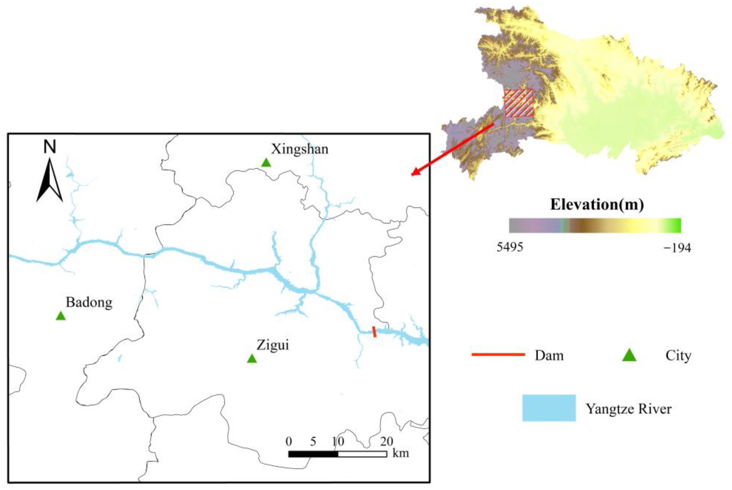
The research area depicted in Figure 1 primarily focuses on the three regions—Badong, Zigui, and Xingshan(HuBei Province, China)—which respond most rapidly to changes in the water-level data upstream of the Three Gorges. This area is located in the upper reaches of the Yangtze River, closest to the Three Gorges Dam and at the dam area of the Three Gorges Reservoir. Meteorological data such as rainfall and temperature, as well as changes in basin conditions, significantly impact the water-level changes in the dam area of the Yangtze River. The annual rainfall in the Three Gorges area is about 1100–1300 mm, with an average yearly temperature of around 18–19 °C. The basins of these three regions cover important tributaries, and their basins are in the dam area of the Three Gorges Reservoir, representing the central dam area region.
2.2. Deep-Learning Models
This study used advanced deep-learning models to accurately predict the water level in the Three Gorges Reservoir and optimize water resource management and disaster warning systems. Specifically, the focus was on exploring four models: Long Short-Term Memory Networks (LSTM), Bidirectional Long Short-Term Memory Networks (BiLSTM), Convolutional Neural Networks combined with Long Short-Term Memory Networks (CNN–LSTM), and Convolutional Neural Network–Attention–Long Short-Term Memory Networks (CNN–Attention–LSTM). These models analyze the water-level data of the Three Gorges Reservoir and consider related data such as inflow, outflow, and rainfall to improve the accuracy and efficiency of water-level predictions [36].
The research focused on the CNN–LSTM and CNN–Attention–LSTM models, designed to address the challenges of predicting water levels in large reservoirs. The CNN–LSTM model integrates the ability of convolutional neural networks to process spatial features with the advantage of long- and short-term memory networks in analyzing time series data. The CNN–Attention–LSTM model further identifies and focuses on crucial information in time series data through the attention mechanism, expecting breakthroughs in improving the accuracy of predicting complex hydrological events. While this model has shown potential in other hydrological prediction fields, such as groundwater-level prediction, its application in predicting water levels in large reservoirs is still novel and warrants an in-depth investigation. This study used a detailed analysis and experimentation to explore the application value and potential of the CNN–Attention–LSTM model in predicting water levels in large reservoirs [37].
2.2.1. LSTM (Long Short-Term Memory) and BiLSTM (Bidirectional Long Short-Term Memory)
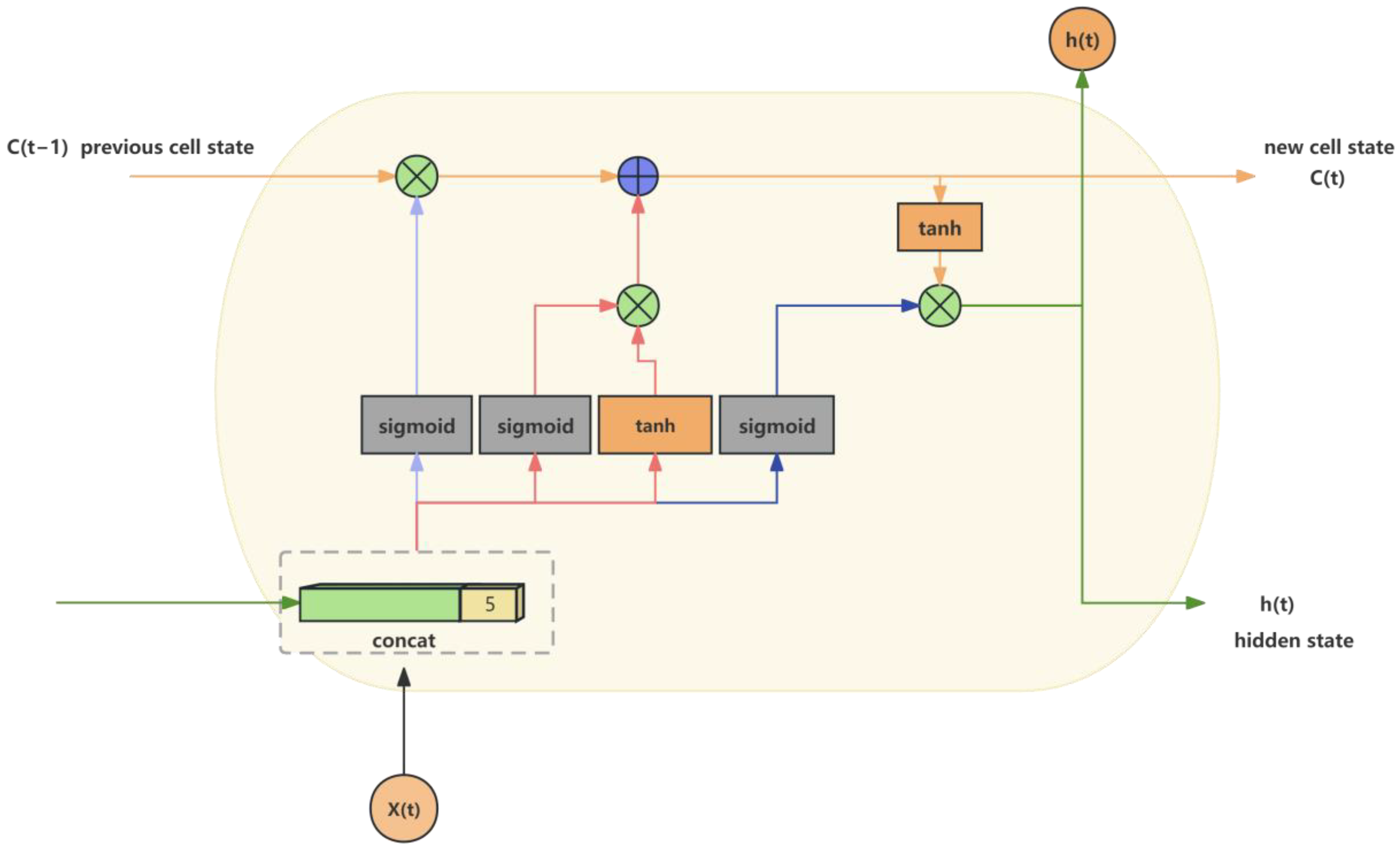
LSTM (Long Short-Term Memory Networks) is a type of Recurrent Neural Network (RNN) specifically designed to address the vanishing and exploding gradients encountered by traditional RNNs when processing long sequences. It effectively manages the storage, updating, and use of information by introducing memory cells () and three critical gating mechanisms, forget gate ), input gate (), and output gate (), allowing the network to capture long-term dependencies. Figure 2 shows the basic network framework of LSTM.
The memory cell is the core of the LSTM network and is responsible for carrying important information throughout the time series. Its update is determined by the following equation:
In Equation (1), is the cell state at the current time step. is the cell state at the previous time step. represents element-wise multiplication, also known as the Hadamard product. The update of the memory cell is a combination of old information controlled by the forget gate and new information controlled by the input gate.
The input gate primarily functions to control the flow of new information into the memory cell. It consists of two parts: a Sigmoid layer, which decides which values need to be updated, and a tanh layer, which creates a new candidate vector to be added to the memory cell. The main equations are
In Equations (2) and (3), is the output of the input gate, and is the new candidate value to be added to the cell state. and are the weight matrices for the input gate and candidate value vector, respectively, while and are their bias terms for the input gate and candidate value vector, respectively.
The forget gate controls the amount of information discarded from the cell state. It decides which information to retain by observing the current input and the previous hidden state:
In Equation (4), is the output of the forget gate at time step t, is the weight matrix of the forget gate, is the hidden state of the previous time step, is the input at the current time step, and is the bias term of the forget gate. is the sigmoid activation function, outputting a number between 0 and 1, indicating how much of the previous time step’s cell state should be retained.
The output gate’s main function is to control the flow of information from the memory cell to the hidden state. Observing the current input and the previous time step’s hidden state and then using the sigmoid function determines which information can be output as the secret state of the current time step. After processing the memory cell through tanh, its output is multiplied by the output gate to obtain the final hidden state .
In Equations (5) and (6), is the output of the forget gate at time step t. is the weight matrix of the forget gate. tanh is the hyperbolic tangent function. is the bias term for the output gate, and is the sigmoid activation function.
BiLSTM (Bidirectional Long Short-Term Memory) extends the traditional LSTM model to enhance its ability to process time series data. Unlike LSTM, which only considers historical information, BiLSTM processes both forward and backward time series data in parallel, effectively integrating the bidirectional contextual details of the sequence. This model deploys two independent hidden states at each time point, learning from both the sequence’s forward (future) and backward (past) directions, thereby achieving a comprehensive analysis of the time series data [38]. This mechanism enables BiLSTM to make predictions based on past data and utilizes an understanding of future trends, thereby improving the accuracy of predictions.
Especially in the field of water-level predictions, the forward hidden layer of the BiLSTM model captures contextual information in the future direction. Even without actual future data, the model can predict potential changes in water levels under specific environmental conditions by analyzing patterns and trends in historical data. For example, the model can identify the pattern of water-level rises within a season and predict future water-level changes under similar seasonal conditions [39].
Furthermore, the bidirectional contextual understanding ability of BiLSTM is particularly suitable for dealing with complex hydrological events, responding to large environmental fluctuations, and predicting sudden events. By utilizing both past and future information, the model provides a deeper understanding of long-term dependencies, significantly improving the accuracy of predictions for complex hydrological phenomena. Therefore, applying the BiLSTM model in water resource management and disaster warning systems enhances predictive performance and provides more reliable support for related decisions [40].
2.2.2. CNN–LSTM Model
This paper introduces a hybrid model combining Convolutional Neural Networks (CNN) and Long Short-Term Memory (LSTM) models to improve the accuracy of predictions. Figure 3 shows the network structure of CNN–LSTM. The CNN–LSTM model leverages the advantage of CNN in feature extraction by automatically detecting and extracting spatial features in time series data through its convolutional layers. These features can be closely related to reservoir water levels. Subsequently, these feature outputs are used as inputs to LSTM, which specializes in handling dependencies, long-term trends, and periodicities in time series data. Compared to the LSTM model, the CNN–LSTM hybrid model can more effectively handle the nonlinear spatial and temporal relationships in the water-level data. Particularly when the dataset has multi-feature inputs, CNN–LSTM can capture medium- and short-term fluctuations and seasonal variations in complex hydrological systems, demonstrating better predictive accuracy and robustness.
The CNN component is primarily situated at the model’s frontend and is responsible for extracting feature variables from the input data. The CNN model is divided into convolutional layers and pooling layers. The convolutional layers are used to extract features at different levels. In contrast, the pooling layers reduce the dimensionality of the features, thus decreasing the computational load of the model. The convolution operation can be represented as
In Equation (7), is the input feature, is the weight of the convolution kernel, is the bias term, represents the convolution operation, is the activation function, and is the output of the convolution layer. The pooling operation is described as
In Equation (8), is the element at position (i, j) in the output of the pooling layer, and is the element within the covered area of the input feature map. The function represents taking the maximum value within the covered area.
The LSTM part is mainly located at the backend of the model, tasked with processing the feature variables captured by the CNN. It captures these feature variables’ dynamic changes and long-term dependencies over a time series.
2.3. CNN–Attention–LSTM
The model is a hybrid neural network that integrates Convolutional Neural Networks (CNNs), Long Short-Term Memory (LSTM), and attention mechanisms designed to solve time series prediction problems, such as water-level forecasting. Figure 4 shows the structure of this network model. By incorporating the attention mechanism, the model can identify and focus on the most critical time points for prediction, especially excelling in handling periodic and seasonal variations. Introducing the attention mechanism enhances the model’s performance and improves its interpretability, making capturing crucial time series features more accurate.
The core advantages of the attention mechanism include
- Selective Attention: Allows the model to focus on crucial information in the sequence dynamically.
- Dynamic Weight Adjustment: Dynamically calculates and adjusts weights based on the prediction task.
- Context Information Integration: This helps the model build a comprehensive context representation, which is crucial for essential prediction information.
- Enhanced Interpretability: Explicitly indicates the parts of the sequence that the model focuses on through attention weights.
The model employs the self-attention mechanism, which is highly suitable for sequence prediction. It can establish dependencies directly between elements within the sequence, capturing long-distance interactions without relying on structures like convolution. The implementation steps of self-attention are as follows:
(1) Compute Query (Q), Key (K), and Value (V): For the features in the sequence, the model learns to generate three particular vectors Q, K, and V through learned linear transformations:
In Equations (9) and (10), represents the input sequence, and are the weight matrices.
(2) Compute Attention Scores: The model calculates the similarity between Q and all Ks. The similarity scores determine the weights for each V:
(3) Calculate the Weighted Sum of Values: The model computes the weighted sum of the value vectors, with weights obtained from the attention scores:
In Equation (13), is the dimension of the critical vector, which is used to scale the dot product to prevent tremendous dot-product values from causing the softmax function’s gradient to be too small.
Introducing the self-attention mechanism significantly enhances the CNN–LSTM model’s ability to understand and process time series data, particularly in recognizing and utilizing temporal features. This improvement increases the model’s predictive accuracy and generalization ability.
Model Design
In all models, the past 36 h of water-level data from the Three Gorges Reservoir (data recorded every six hours, with four observations per day), the difference in inflow and outflow rates, and rainfall data from the three main upstream areas (Badong, Zigui, and Xingshan) are used as inputs, with a dimension of [19,124, 6, 5] (19,124 input data, 6 for the sliding window, and 5 for the number of features). The LSTM and BiLSTM models are configured with two layers, each with 128 units. For the CNN–LSTM model, three layers of convolutional networks are designed to extract spatiotemporal features, a max-pooling layer after each layer, and then two layers of LSTM units. The CNN–Attention–LSTM model adds a self-attention layer on this basis to enhance the model’s ability to recognize key timestep features.
The model training uses the Adam optimizer, with an initial learning rate of 0.0001. The batch size is 64, with an average training of 392 epochs. To prevent overfitting, the model also employs early stopping, monitoring the loss on the validation set, and stopping training if there is no improvement over ten consecutive epochs. The specific parameters of each model can be found in Table 1.
In this study, the model’s input parameters include the water-level data of the Three Gorges Reservoir over a past period, the difference in inflow and outflow rates, and rainfall data. The output parameter is the predicted water level for a particular future time range. Specifically, the past 36 h of data are used as input to indicate water-level changes within the next 6 h.
To assess the impact of different retrospective periods on model performance, the experiment tested three different retrospective period settings: 24 h, 36 h, and 48 h. The results showed that a 36 h retrospective period provided the highest prediction accuracy, while longer or shorter retrospective periods led to a decline in performance. This finding emphasizes the importance of the length of the retrospective period in time series prediction models. It highlights the necessity of finding the optimal retrospective period for specific prediction tasks.
To achieve this goal, each hour’s data for a year are divided according to a 36 h retrospective period, with each data sequence containing 36 h of continuous input data, followed by the next 6 h as the prediction target. This method constructs multiple input-output sequence pairs, each corresponding to the historical data within a specific retrospective period and the predicted future water level. This data division strategy considers the continuity of the time series. It fully utilizes historical water-level data, flow rate difference, and rainfall information, thereby enhancing the model’s ability to capture future water-level trends.
2.4. Data Preprocessing
2.4.1. Data Selection
The primary data selected for this study include reservoir head area water-level data and inflow and outflow velocities from 1 January 2008 to 1 February 2021. The data were collected at six-hour intervals, totaling 19,124 data entries. Rainfall data were obtained from Badong, Zigui, and Xingshan hydrometeorological stations. The information shown in Table 2 is for three hydrological stations. As the primary feature data, the outflow and inflow velocities of the Three Gorges Reservoir area were selected. The model calculates these two data points into a single feature data that has a more significant impact on the water level:
In Equation (14), represents the net inflow into the reservoir (positive values indicate inflow, while negative values indicate outflow), represents the inflow velocity, represents the outflow velocity, and is the time interval between each data point.

Table 2.
Parameter information of hydrological and meteorological stations.
| Hydrometeorological Station | District Station Number | Longitude | Latitude | Altitude (m) |
|---|---|---|---|---|
| BaDong | 57,355 | 31.02 | 110.22 | 334.0 |
| ZiGui | 57,461 | 30.44 | 111.22 | 256.5 |
| XingShan | 57,359 | 31.21 | 110.44 | 336.8 |
2.4.2. Data Normalization
Rainfall data and the difference in water-level flow velocities are inputs. Different data metrics scales can affect the training model’s convergence speed and reliability. In this model, min–max normalization is applied, a technique that scales values from 0 to 1. The primary purpose of this technique is to eliminate the impact of different scales among data features, allowing each feature value to be computed on the same scale and enhancing the algorithm’s accuracy and the model’s convergence speed.
In Equation (15), represents the original data, and and are the minimum and maximum values of the data for that particular feature, respectively.
2.4.3. Dataset Division
To ensure the effectiveness of the model training and accurately assess its generalization ability, the entire dataset is divided into three independent subsets: training set, test set, and validation set. The data are allocated in an 8:1:1 ratio, initially divided into sequential blocks in chronological order, with 80% of the data used for training the model. This portion helps the model learn and adjust its internal parameters. The remaining 20% of the data are evenly distributed between the test and validation sets, each comprising 10%. The validation set is used for model tuning and hyperparameter selection, while the test set is utilized to evaluate the model’s performance on unseen data. This division ratio ensures sufficient data for training the model while effectively validating and testing the model’s generalization ability, providing a more accurate understanding of the model’s strengths and limitations.
2.5. Model Establishment and Evaluation Criteria
In evaluating model performance, this study primarily utilized metrics such as R2, MAE, RMSE, and MAPE, chosen for their widespread recognition and effectiveness in hydrological and environmental model analysis. These metrics comprehensively reflect the predictive capacity of the model and consider both the magnitude and distribution of errors, thereby providing a solid foundation for assessing and comparing the performance of different models. The Nash–Sutcliffe efficiency coefficient E, Relative Root Mean Square Error (RRSE), and Percent Bias (PBIAS) mentioned by Alicante [41] in a study on an irrigation network flow model calibration in Spain suggest that these indicators are worth considering for future research due to their specific advantages. However, given the goals of this study and the characteristics of the data handled, the combined application of R2, MAE, RMSE, and MAPE better meets the dual needs of this research for prediction accuracy and error sensitivity.
R2 (Coefficient of Determination): It measures the degree to which the model explains the variability of the data. It represents the proportion of explained variation to the total variation. R2 values usually range between 0 and 1, with values closer to 1 indicating the model’s more substantial explanatory power. The formula for R2 is
MAE (Mean Absolute Error): It measures the average magnitude of the absolute differences between predictions and actual observations, giving an average level of prediction error:
RMSE (Root Mean Square Error) is the square root of the average of the squared differences between observed values and model predictions. It gives greater weight to larger errors, penalizing them more heavily:
MAPE (Mean Absolute Percentage Error): It measures the size of the prediction error compared to the actual value, usually expressed in percentage form, providing an intuitive representation of the relative size of the error:
In Equations (16)–(19), is the observed value, is the predicted value by the model, and is the average of the observed values.
3. Experimental Results Analysis
To evaluate the model’s overall performance, it is essential to consider its overall fit, generalization ability, and robustness. The original data, including the water-level difference in the Three Gorges Reservoir head area and the rainfall in Badong, Zigui, and Xingshan, were divided into training, testing, and validation sets in an 8:1:1 ratio. The predicted values from the LSTM, BiLSTM, CNN–LSTM, and CNN–Attention–LSTM models were compared. The performance of each model on the validation set is as follows:
From Table 3 and Table 4, the evaluation metrics of the models show that the BiLSTM and CNN–LSTM models, compared to the LSTM model, have improved R2 from 0.9635 to 0.9689 and 0.9883, respectively, an increase of 0.56% and 2.57%. This indicates that the two models have improved in explaining water-level changes compared to LSTM and can better capture the changing trends and patterns in the data. The MAE decreased from 1.3841 to 1.2724 and 0.7920, a percentage improvement of 8.07% and 42.78%, respectively. The RMSE decreased from 1.6721 to 1.5427 and 0.9484, a percentage improvement of 7.74% and 43.3%, respectively. Since RMSE is more sensitive to differences, the results indicate that the two models are more effective in handling extreme values and peaks in water-level data. The MAPE decreased from 0.0082 to 0.0073 and 0.0047, a percentage improvement of 10.98% and 42.68%, respectively, indicating that the two models significantly improved prediction accuracy compared to LSTM.
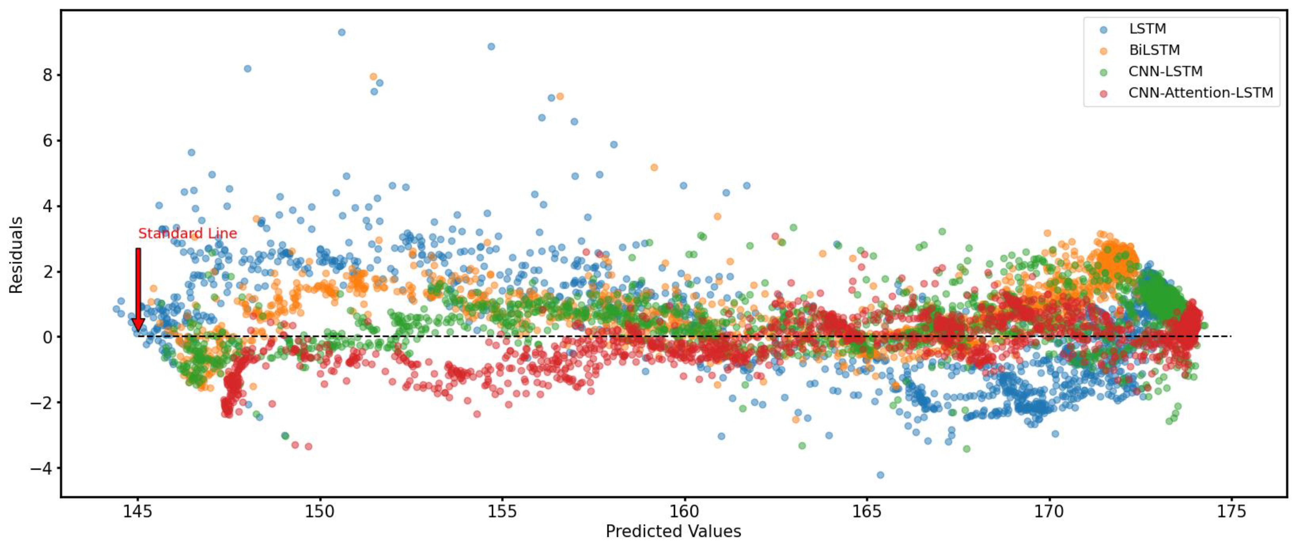
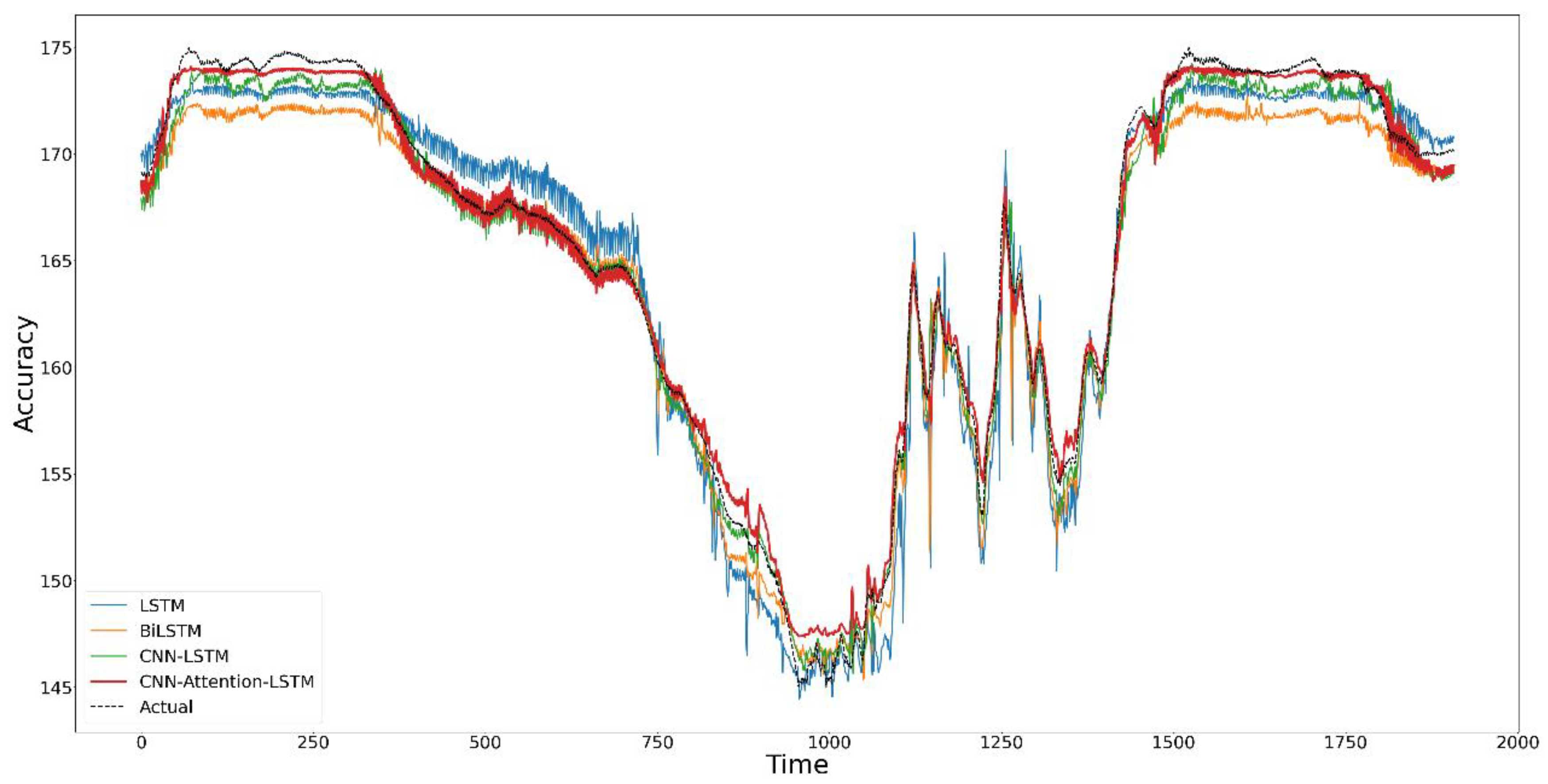
The results show that BiLSTM, by considering forward and backward information on water levels and learning from both past and future data, has improved overall evaluation metrics. It can understand the dynamic changes in hydrological data more comprehensively. Compared to LSTM, BiLSTM has demonstrated a more vital predictive ability in handling water-level data with complex temporal dependencies. Figure 8 shows that the LSTM’s predictions are higher than the actual values for water levels below 160 m and lower than those above 160 m. Figure 9 shows that the BiLSTM model’s predicted values are more closely aligned with the actual values. However, the prediction ability for peak water levels (above 170 m or below 150 m) is relatively poor, which is also why the RMSE did not significantly improve.The BiLSTM model is more balanced overall, indirectly indicating that the model has more substantial prediction stability.
Compared to the other two models, the CNN–LSTM model shows improvements across all metrics, attributable to the spatial feature extraction capability of CNN and LSTM’s strength in handling time series data. After the CNN component identifies spatial features in rainfall data and flow changes, the LSTM part effectively captures these features as they evolve over time. This model is more effective in processing complex features related to water-level changes. CNN mainly plays the role of feature extraction in the model, extracting relevant vital features, allowing LSTM to more accurately capture and analyze factors affecting water-level changes in the time series. The overall improvement in performance suggests that the CNN–LSTM model exhibits better generalization ability and stability and accuracy in complex environments. It can somewhat reduce the impact of data noise and outliers, enhancing predictive accuracy.
From Figure 9, it is evident that the CNN–LSTM model can accurately predict the fluctuations in water levels, with a noticeable improvement in predicting peak values. The prediction curve closely aligns with the actual value curve. In Figure 8, it can be observed that the CNN–LSTM model predictions hover around the zero line, significantly reducing large positive residuals (where actual values are much greater than predicted values) and harmful residuals (where exact values are much less than predicted values). This reaffirms the CNN–LSTM model’s enhanced capability in predicting outliers and sudden hydrological events.
Table 5 shows that the CNN–LSTM model, with the addition of the attention mechanism, significantly improves the model’s ability to predict water levels. In terms of performance evaluation, the CNN–LSTM model optimized with the attention mechanism has been enhanced by 0.57%, 33.13%, 28.84%, and 31.91% in the four evaluation metrics: R2, MAE, RMSE, and MAPE. From Figure 9, it can be observed that the predicted curve can fuse better with the true value curve compared to the CNN–LSTM model. This indicates that the CNN–Attention–LSTM model can better explain water-level data, suggesting a closer correlation between actual and predicted values. The introduction of the attention mechanism effectively guides the factors that have the most significant impact on the prediction results, thereby reducing prediction errors. The overall improvement in RMSE indicates that the model is more accurate, especially in handling extreme values and peaks. Compared to the CNN–LSTM model, the model with the attention mechanism can more effectively identify and utilize critical information in feature values, especially the improvement in peak prediction accuracy, indicating that the model with the attention mechanism can better capture critical factors affecting water levels, such as sudden rainfall events or seasonal flow changes when analyzing instantaneous and seasonal hydrological changes.
In this study, the actual values presented in Figure 9 and Figure 10 originate from real observational data collected at hydrological monitoring stations. The forecast values depicted are not generated through extended model runs; that is, this study did not use the predictions from a previous time point as inputs to continuously forecast future states. Each data point shown is independent of model predictions and directly reflects the actual observations.
Overall, in Figure 9, the prediction curve of the CNN–Attention–LSTM model is closest to the actual value curve, performing best among all models. Figure 10 shows that the model with the attention mechanism performs better in peak predictions above 170 m water levels. Still, in peak predictions below 150 m water levels, the CNN–LSTM model performs better. It can also be seen in Figure 8 that, except for low-water-level predictions, the overall prediction of the CNN–Attention–LSTM model is of a higher standard.
An in-depth analysis of the Three Gorges Reservoir water-level-prediction models, primarily focusing on the performance of CNN–LSTM and CNN–Attention–LSTM models under conditions where water levels are above 170 m and below 150 m, shows that when water levels are above 170 m, the Coefficient of Determination (R2 value) of the CNN–Attention–LSTM model significantly increases to 0.861, much higher than the 0.399 of the CNN–LSTM model. This result highlights the effectiveness and importance of the attention mechanism in extremely high-water-level prediction. Conversely, in scenarios where water levels are below 150 m, the CNN–LSTM model surpasses the CNN–Attention–LSTM model with an R2 value of 0.695 compared to 0.563. This comparison reflects that although the attention mechanism significantly improves the prediction ability for high-water-level changes, it may fail to effectively capture key features in low-water-level-prediction scenarios, leading to reduced performance. This suggests that during further model improvement, it is necessary to refine and adjust the application strategy of the attention mechanism for different water-level conditions.
Exploring the phenomenon of improved prediction accuracy for high water levels (>170 m) and reduced accuracy for low water levels (<150 m) after adding the attention mechanism to the CNN–LSTM model may involve several vital factors. First, distribution bias in the dataset may make the features of high-water-level samples more consistent and prominent, which are quickly learned by the attention mechanism as these frequent and distinct cases ignore the dispersed features of low-water-level samples. Second, introducing the attention mechanism may cause the model to overly focus on significant features of high water levels, failing to fully identify essential information under low-water-level conditions. Additionally, the model may experience overfitting during the training process, especially in over-optimizing high-water-level data, which affects its generalization ability for low-water-level situations. Lastly, differences in environmental influences under different water-level conditions may also be a factor, as environmental features during high-water-level periods may be more uniform. Various factors may affect low-water-level periods, increasing the complexity of prediction. The combined effects of these factors lead to differences in model prediction performance across different water-level intervals, emphasizing the importance of considering data distribution, feature complexity, and environmental factors in model design and training.
During the prediction process, the attention mechanism enhances the model’s robustness to outliers and noise, meaning that the model can maintain high prediction accuracy even in imperfect data quality. The improvement in various evaluation metrics proves that the CNN–LSTM model with the attention mechanism has become a powerful tool for predicting water levels in the Three Gorges Reservoir area.
4. Conclusions
This study conducts a deep comparison of different deep-learning models applied to water-level predictions in the Three Gorges Reservoir, focusing on Long Short-Term Memory Networks (LSTM), Bidirectional Long Short-Term Memory Networks (BiLSTM), the combination of Convolutional Neural Networks and Long Short-Term Memory Networks (CNN–LSTM), and the CNN–LSTM model further incorporating the attention mechanism (CNN–Attention–LSTM). Through a detailed analysis of the performance of the models on critical metrics, it was found that the CNN–LSTM model showed significant improvement in prediction accuracy compared to the LSTM and BiLSTM models, and the CNN–LSTM model with the attention mechanism enhanced predictive capabilities.
Especially in large-scale hydraulic structures like the Three Gorges Reservoir, an accurate water-level prediction is crucial for flood control, optimal allocation of water resources, and ecological protection. Our research emphasizes the practical value of deep-learning models in these critical applications, demonstrating how these models can be utilized to handle vast amounts of complex hydrological data to provide more precise forecasts and decision support. The methodology highlighted the ability of deep-learning technology to handle complex spatiotemporal sequence data, especially the role of the attention mechanism in enhancing the model’s ability to capture essential information.
The results revealed a clear improvement in the BiLSTM and CNN–LSTM models compared to the LSTM model in terms of R2, MAE, RMSE, and MAPE metrics due to the bidirectionality of BiLSTM. In particular, the CNN–LSTM model, by combining the spatial feature extraction advantage of CNN and the temporal series analysis capability of LSTM, demonstrated better generalization ability and adaptability to complex environments. Furthermore, the CNN–LSTM model, with the addition of the attention mechanism, showed further performance improvements in all evaluation metrics, proving the effectiveness of the attention mechanism in enhancing the model’s accuracy in water-level predictions. Experimental results showed that the CNN–LSTM model performed excellently in handling complex features related to water-level changes, showing the best results in predicting low water levels. At the same time, introducing the attention mechanism allowed the model to more accurately predict fluctuations in water levels, especially in predicting high-water-level peaks.
This research demonstrated significant advantages of applying deep-learning technology in predicting water levels in the Three Gorges Reservoir, especially the performance improvement obtained by combining CNN and LSTM models and further introducing the attention mechanism. These findings emphasize the importance of comprehensively utilizing multi-source data and reveal the necessity of customizing model structures and parameter optimization for specific prediction tasks. Future research directions include exploring different attention mechanisms to improve model accuracy, enhancing model interpretability and transparency, and developing dynamic models that can adapt to new data in real time. Furthermore, considering the long-term impact of climate change, research on long-term water-level-prediction models that incorporate climate model predictions as inputs will be of significant value. Through these efforts, the accuracy and efficiency of water-level predictions can be further improved, and more effective support can also be provided for water resource management, disaster early warning, and adaptation to climate change.
In summary, this study demonstrated the application value of deep-learning models, especially the CNN–LSTM model, in predicting water levels in the Three Gorges Reservoir and showed how the attention mechanism effectively enhances the model’s predictive capabilities. These findings provide new technical paths for hydrological prediction and have essential theoretical and practical significance for optimizing reservoir management and improving flood control decision support systems. Future research can further explore the application of deep-learning technology in hydrology and related fields, especially regarding the potential to improve model prediction capabilities for exceptional events. This study not only provides efficient and reliable deep-learning methods for water-level predictions in large-scale hydraulic facilities like the Three Gorges Reservoir but also lays a theoretical and practical foundation for the broader application of deep-learning technology in hydrology and environmental science. By continuing to push the boundaries of technology, we can better address the challenges posed by global climate change, offering robust scientific support for sustainable water resource management and disaster prevention.
Author Contributions
Software, H.L.; Formal analysis, R.W.; Data curation, Y.Z.; Writing—original draft, H.L.; Writing—review & editing, L.Z.; Visualization, H.L.; Project administration, Y.D.; Funding acquisition, L.Z. and Y.Y. All authors have read and agreed to the published version of the manuscript.
Funding
This study is financially supported by the Science and Technology Innovation Program for Postgraduate students in IDP subsidized by Fundamental Research Funds for the Central Universities (Granted No. ZY20240336), by the National Natural Science Foundation of China (Granted Nos. 41702264 and 42174177), and by the China Three Gorges Corporation Program (Granted No. 0799217).
Data Availability Statement
The data supporting this study’s findings are available from the corresponding author upon reasonable request.
Conflicts of Interest
The authors declare no conflict of interest.
References
- Jiang, L.Z.; Ban, X.; Wang, X.L.; Cai, X.B. Assessment of Hydrologic Alterations Caused by the Three Gorges Dam in the Middle and Lower Reaches of Yangtze River, China. Water 2014, 6, 1419–1434. [Google Scholar] [CrossRef]
- Zhang, X.; Dong, Z.; Gupta, H.; Wu, G.; Li, D. Impact of the Three Gorges Dam on the hydrology and ecology of the Yangtze River. Water 2016, 8, 590. [Google Scholar] [CrossRef]
- Wu, C.L.; Chau, K.W.; Li, Y.S. Predicting monthly streamflow using data-driven models coupled with data-preprocessing techniques. Water Resour. Res. 2009, 45. [Google Scholar] [CrossRef]
- Huang, S.; Chang, J.; Huang, Q.; Chen, Y. Monthly streamflow prediction using modified EMD-based support vector machine. J. Hydrol. 2014, 511, 764–775. [Google Scholar] [CrossRef]
- Lee, T.; Ouarda, T.B.M.J. Long-term prediction of precipitation and hydrologic extremes with nonstationary oscillation processes. J. Geophys. Res. 2010, 115, D13107. [Google Scholar] [CrossRef]
- Huang, A.N.; Yerubandi, R.R.; Lu, Y.Y.; Zhao, J. Hydrodynamic modeling of Lake Ontario: An intercomparison of three models. J. Geophys. Res. 2010, 115, C12076. [Google Scholar] [CrossRef]
- Vahid, M.; Bideskan, M.E.; Behbahani, S.M.R. Parameters Estimate of Autoregressive Moving Average and Autoregressive Integrated Moving Average Models and Compare Their Ability for Inflow Forecasting. J. Math. Stat. 2012, 8, 330–338. [Google Scholar]
- Zhu, S.; Zhou, J.; Ye, L.; Meng, C. Streamflow estimation by support vector machine coupled with different methods of time series decomposition in the upper reaches of Yangtze River, China. Environ. Earth Sci. 2016, 75, 531. [Google Scholar] [CrossRef]
- Wang, W.C.; Chau, K.W.; Qiu, L.; Chen, Y.B. Improving forecasting accuracy of medium and long-term runoff using artificial neural network based on EEMD decomposition. Environ. Res. 2015, 139, 46–54. [Google Scholar] [CrossRef]
- Breiman, L. Bagging predictors. Mach. Learn. 1996, 24, 123–140. [Google Scholar] [CrossRef]
- Friedman, J.H. Greedy function approximation: A gradient boosting machine. Ann. Stat. 2001, 29, 1189–1232. [Google Scholar] [CrossRef]
- Friedman, J.H. Stochastic gradient boosting. Comput. Stat. Data Anal. 2002, 38, 367–378. [Google Scholar] [CrossRef]
- Vahid, M. Predicting Caspian Sea surface water level by ANN and ARIMA models. J. Waterw. Port Coast. Ocean. Eng. 1997, 123, 158–162. [Google Scholar]
- Xu, G.Y.; Cheng, Y.; Liu, F.; Ping, P.; Sun, J. A Water Level Prediction Model Based on ARIMA-RNN. In Proceedings of the 2019 IEEE Fifth International Conference on Big Data Computing Service and Applications (BigDataService), Newark, CA, USA, 4–9 April 2019; IEEE: New York, NK, USA, 2019. [Google Scholar] [CrossRef]
- Anctil, F.; Lauzon, N. Generalisation for neural networks through data sampling and training procedures with applications to streamflow predictions. Hydrol. Earth Syst. Sci. 2004, 8, 940–958. [Google Scholar] [CrossRef]
- Snelder, T.H.; Lamouroux, N.; Leathwick, J.R.; Pella, H.; Sauquet, E.; Shankar, U. Predictive mapping of the natural flow regimes of France. J. Hydrol. 2009, 373, 57–67. [Google Scholar] [CrossRef]
- Mekanik, F.; Imteaz, M.A.; Gato-Trinidad, S.; Elmahdi, A. Multiple regression and Artificial Neural Network for long-term rainfall forecasting using large scale climate modes. J. Hydrol. 2013, 503, 11–21. [Google Scholar] [CrossRef]
- Xu, Z.X.; Li, J.Y. Short-term inflow forecasting using an artificial neural network model. Hydrol. Process. 2002, 16, 2423–2439. [Google Scholar] [CrossRef]
- Graves, A.; Graves, A. Long short-term memory. Supervised Seq. Label. Recurr. Neural Netw. 2012, 37–45. [Google Scholar] [CrossRef]
- Liu, X.Y.; Yao, H.M.; Zhang, H.R. Machine learning based hourly scale water level prediction in front of the Three Gorges Reservoir dam. Yangtze River 2023, 54, 147–151. [Google Scholar]
- de la Fuente, A.; Meruane, V.; Meruane, C. Hydrological early warning system based on a deep learning runoff model coupled with a meteorological forecast. Water 2019, 11, 1808. [Google Scholar] [CrossRef]
- Hrnjica, B.; Bonacci, O. Lake level prediction using feed-forward and recurrent neural networks. Water Resour. Manag. 2019, 33, 2471–2484. [Google Scholar] [CrossRef]
- Baek, S.-S.; Pyo, J.; Chun, J.A. Prediction of water level and water quality using a CNN-LSTM combined deep learning approach. Water 2020, 12, 3399. [Google Scholar] [CrossRef]
- Pan, M.; Zhou, H.; Cao, J.; Liu, Y.; Hao, J.; Li, S.; Chen, C.-H. Water level prediction model based on GRU and CNN. IEEE Access 2020, 8, 60090–60100. [Google Scholar] [CrossRef]
- Zhang, Y.; Zhou, Z.; Van Griensven Thé, J.; Yang, S.X.; Gharabaghi, B. Flood Forecasting Using Hybrid LSTM and GRU Models with Lag Time Preprocessing. Water 2023, 15, 3982. [Google Scholar] [CrossRef]
- Nie, Q.; Wan, D.; Wang, R. CNN-BiLSTM water level prediction method with attention mechanism. J. Phys. Conf. Ser. 2021, 2078, 012032. [Google Scholar] [CrossRef]
- Shen, C. A transdisciplinary review of deep learning research and its relevance for water resources scientists. Water Resour. Res. 2018, 54, 8558–8593. [Google Scholar] [CrossRef]
- Karim, S.M.H.I.; Yuk, F.H.; Ali, N.A.; Chai, H.K.; Ahmed, E.S. A review of the hybrid artificial intelligence and optimization modeling of hydrological streamflow forecasting. Alex. Eng. J. 2022, 61, 279–303. [Google Scholar]
- Xie, Z.Q.; Liu, Q.; Cao, Y.L. Hybrid Deep Learning Modeling for Water Level Prediction in Yangtze River. Intell. Autom. Soft Comput. 2021, 28, 153–166. [Google Scholar] [CrossRef]
- Yin, H.; Li, C. Human impact on floods and flood disasters on the Yangtze River. Geomorphology 2001, 41, 105–109. [Google Scholar] [CrossRef]
- Sarah, S.J.M.; Salah, L.Z.; Sandra, O.M.; Nadhir, A.A.; Saleem, E.; Khalid, H. Application of hybrid machine learning models and data pre-processing to predict water level of watersheds: Recent trends and future perspective. Cogent Eng. 2022, 9, 2143051. [Google Scholar] [CrossRef]
- Wu, J.; Huang, J.; Han, X.; Gao, X.; He, F.; Jiang, M.; Shen, Z. The Three Gorges Dam: An ecological perspective. Front. Ecol. Environ. 2004, 2, 241–248. [Google Scholar] [CrossRef]
- Zhang, Q.; Lou, Z. The environmental changes and mitigation actions in the Three Gorges Reservoir region, China. Environ. Sci. Policy 2011, 14, 1132–1138. [Google Scholar] [CrossRef]
- Tang, H.; Wasowski, J.; Juang, C.H. Geohazards in the Three Gorges Reservoir Area, China–Lessons learned from decades of research. Eng. Geol. 2019, 261, 105267. [Google Scholar] [CrossRef]
- Yang, Y.; Guo, H.; Chen, L.; Liu, X.; Gu, M.; Pan, W. Multiattribute decision making for the assessment of disaster resilience in the Three Gorges Reservoir Area. Ecol. Soc. 2020, 25, 75. [Google Scholar] [CrossRef]
- Hiu, J.A.; Shiv, F.C.; Bogdan, O.P.; Anna, O.-Z. Comparison of multiple linear and nonlinear regression, autoregressive integrated moving average, artificial neural network, and wavelet artificial neural network methods for urban water demand forecasting in Montreal, Canada. Water Resour. Res. 2012, 48, W01528. [Google Scholar] [CrossRef]
- Khatibi, R.; Ghorbani, M.A.; Naghipour, L.; Jothiprakash, V.; Fathima, T.A.; Fazelifard, M.H. Inter-comparison of time series models of lake levels predicted by several modeling strategies. J. Hydrol. 2014, 511, 530–545. [Google Scholar] [CrossRef]
- Graves, A.; Jaitly, N.; Mohamed, A. Hybrid speech recognition with Deep Bidirectional LSTM. In Proceedings of the 2013 IEEE Workshop on Automatic Speech Recognition and Understanding, Olomouc, Czech Republic, 8–12 December 2013. [Google Scholar]
- Hochreiter, S.; Schmidhuber, J. Long Short-Term Memory. Neural Comput. 1997, 9, 1735–1780. [Google Scholar] [CrossRef] [PubMed]
- Schuster, M.; Paliwal, K.K. Bidirectional Recurrent Neural Networks. IEEE Trans. Signal Process. 1997, 45, 2673–2681. [Google Scholar] [CrossRef]
- Pérez-Sánchez, M.; Sánchez-Romero, F.J.; Ramos, H.M.; Jiménez, P.A.L. Calibrating a flow model in an irrigation network: Case study in Alicante, Spain. Span. J. Agric. Res. 2017, 15, 1–13. [Google Scholar] [CrossRef]
Figure 1.
Geographical location and water system map of the research area.

Figure 2.
Conceptual diagram of the extended short-term memory model.

Figure 3.
Convolutional Neural Network–Conceptual Graph of Long Short-Term Memory Models.

Figure 4.
Concept diagram of convolutional neural network with attention mechanism added-extended short-term memory model.
Figure 4.
Concept diagram of convolutional neural network with attention mechanism added-extended short-term memory model.

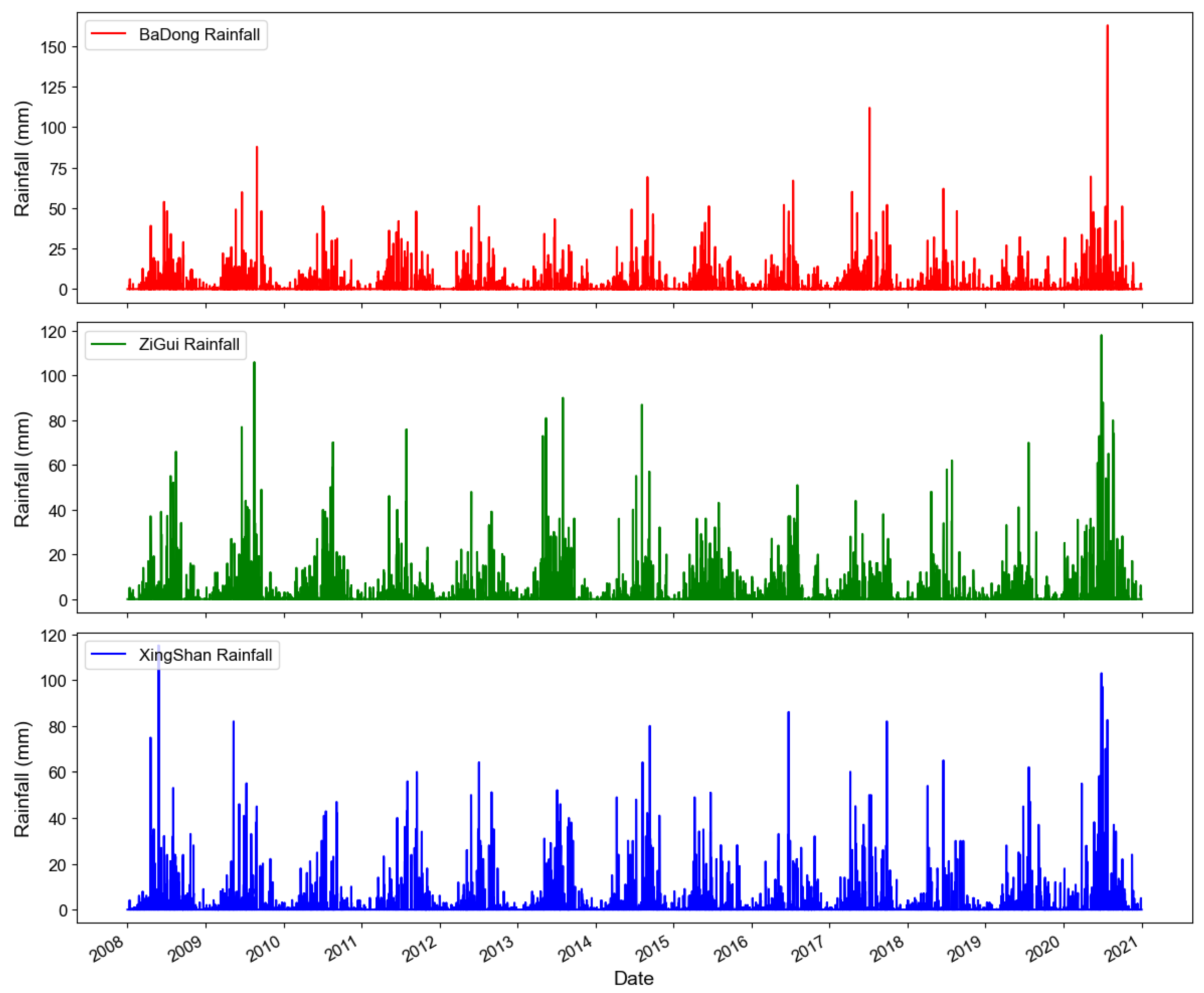
Figure 5.
Rainfall data maps for Badong, Xingshan, and Zigui regions.

Figure 6.
Water-level data map of the head area of the Three Gorges Reservoir.

Figure 7.
Data table of reservoir water flow velocity difference.

Figure 8.
Residual plots of predicted valid values for LSTM, BiLSTM, CNN–LSTM, and CNN–Attention LSTM models.
Figure 8.
Residual plots of predicted valid values for LSTM, BiLSTM, CNN–LSTM, and CNN–Attention LSTM models.

Figure 9.
Comparison chart of predictions by four models: LSTM, BiLSTM, CNN–LSTM, CNN–At tention-LSTM.
Figure 9.
Comparison chart of predictions by four models: LSTM, BiLSTM, CNN–LSTM, CNN–At tention-LSTM.

Figure 10.
Comparison of prediction results between CNN LSTM and CNN–Attention–LSTM models.

Table 1.
Summary Table of Model Parameters.
| Model Type | Input Dimensions | Output Dimensions | Key Layer Composition | Optimizer |
|---|---|---|---|---|
| LSTM | (epoch, 6, 5) | (epoch, 1) | 2× LSTM, 1× Dense | TensorFlow Adam with learning rate of 0.0001 |
| BiLSTM | (epoch, 6, 5) | (epoch, 1) | 2× BiLSTM, 1× Dense | TensorFlow Adam with learning rate of 0.0001 |
| CNN–LSTM | (epoch, 6, 5) | (epoch, 1) | Conv1D, MaxPooling1D, 2× LSTM, 1× Dense | TensorFlow Adam with learning rate of 0.0001 |
| CNN–Attention–LSTM | (epoch, 6, 5) | (epoch, 1) | Conv1D, MaxPooling1D, Attention, 2× LSTM, 1× Dense | TensorFlow Adam with learning rate of 0.0001 |
Table 3.
Performance of Model on the test set.
| Evaluating Indicator | R2 | MAE | RMSE | MAPE |
|---|---|---|---|---|
| LSTM | 0.9635 | 1.3841 | 1.6721 | 0.82% |
| BiLSTM | 0.9689 | 1.2724 | 1.5427 | 0.73% |
| CNN–LSTM | 0.9883 | 0.7920 | 0.9484 | 0.47% |
| CNN–Attention–LSTM | 0.9940 | 0.5296 | 0.6748 | 0.32% |
Table 4.
The degree of performance improvement of BiLSTM and CNN–LSTM compared to LSTM models.
| Improvement Degree | R2 | MAE | RMSE | MAPE |
|---|---|---|---|---|
| LSTM | 0.9635 | 1.3841 | 1.6721 | 0.82% |
| BiLSTM | 0.56% | 8.07% | 7.74% | 10.98% |
| CNN–LSTM | 2.57% | 42.78% | 43.3% | 42.68% |
| CNN–Attention–LSTM | 3.17% | 61.82% | 59.62% | 60.98% |
Table 5.
Performance improvement percentage table of CNN–LSTM model after adding attention mechanism.
Table 5.
Performance improvement percentage table of CNN–LSTM model after adding attention mechanism.
| Improvement Degree | R2 | MAE | RMSE | MAPE |
|---|---|---|---|---|
| CNN–LSTM | 0.9883 | 0.7920 | 0.9484 | 0.47% |
| CNN–Attention–LSTM | 0.57% | 33.13% | 28.84% | 31.91% |
Disclaimer/Publisher’s Note: The statements, opinions and data contained in all publications are solely those of the individual author(s) and contributor(s) and not of MDPI and/or the editor(s). MDPI and/or the editor(s) disclaim responsibility for any injury to people or property resulting from any ideas, methods, instructions or products referred to in the content. |
© 2024 by the authors. Licensee MDPI, Basel, Switzerland. This article is an open access article distributed under the terms and conditions of the Creative Commons Attribution (CC BY) license (https://creativecommons.org/licenses/by/4.0/).
Share and Cite
MDPI and ACS Style
Li, H.; Zhang, L.; Zhang, Y.; Yao, Y.; Wang, R.; Dai, Y. Water-Level Prediction Analysis for the Three Gorges Reservoir Area Based on a Hybrid Model of LSTM and Its Variants. Water 2024, 16, 1227. https://doi.org/10.3390/w16091227
AMA Style
Li H, Zhang L, Zhang Y, Yao Y, Wang R, Dai Y. Water-Level Prediction Analysis for the Three Gorges Reservoir Area Based on a Hybrid Model of LSTM and Its Variants. Water. 2024; 16(9):1227. https://doi.org/10.3390/w16091227
Chicago/Turabian StyleLi, Haoran, Lili Zhang, Yaowen Zhang, Yunsheng Yao, Renlong Wang, and Yiming Dai. 2024. "Water-Level Prediction Analysis for the Three Gorges Reservoir Area Based on a Hybrid Model of LSTM and Its Variants" Water 16, no. 9: 1227. https://doi.org/10.3390/w16091227
Note that from the first issue of 2016, this journal uses article numbers instead of page numbers. See further details here.