


Abstract
Analytical solutions for 2D and slab turbulence energies in the solar corona are presented, including a derivation of the corresponding correlation lengths, with implications for the proton and electron temperatures in the solar corona. These solutions are derived by solving the transport equations for 2D and slab turbulence energies and their correlation lengths, as well as proton and electron pressures. The solutions assume background profiles for the solar wind speed, solar wind mass density, and Alfvén velocity. Our analytical solutions can be related to those obtained from joint Parker Solar Probe and Solar Orbiter Metis coronagraph observations, as reported in Telloni et al. We find that the solution for 2D turbulence energy in the absence of nonlinear dissipation decreases more slowly compared to the dissipative solution. The solution for slab turbulence energy with no dissipation exhibits a more rapid increase compared to the dissipative solution. The proton heating rate is found to be about 82% of the total plasma heating rate at 6.3 R⊙, which gradually decreases with increasing distance, eventually becoming ∼80% of the total plasma heating rate at ∼13 R⊙, consistent with that found by Bandyopadhyay et al. (2023). These analytical solutions provide valuable insight for our understanding of turbulence, and its effect on proton and electron heating rates, in the solar corona. We compare the numerically solved turbulent transport equations for the 2D and slab turbulence energies, correlation lengths, and proton and electron pressures with the analytical solutions, finding good agreement between them.
Export citation and abstract BibTeX RIS

Original content from this work may be used under the terms of the Creative Commons Attribution 4.0 licence. Any further distribution of this work must maintain attribution to the author(s) and the title of the work, journal citation and DOI.
1. Introduction
The corona, the outermost layer in the solar atmosphere, is formed by heated plasma partially confined by strong open and closed magnetic field lines that control the plasma energy and pressure density. The solar corona is heated to temperatures of millions of degrees Kelvin to form the solar wind, whose speed transitions from subsonic to supersonic. Despite extensive research since the late 1950 s (Parker 1958, 1965), understanding the complex mechanisms leading to coronal heating and solar wind acceleration remains a persistent challenge. The launches of the Parker Solar Probe (PSP; Fox et al. 2016) and Solar Orbiter (SO; Müller et al. 2020) have provided in situ observations closer to the Sun than ever before. Recent studies have used the proximity of these two spacecraft to the Sun to advance our understanding of the mechanisms governing solar coronal heating and solar wind generation (Kasper et al. 2021; Telloni et al. 2022b; Zank et al. 2022; Bale et al. 2023; Raouafi et al. 2023).
One of the promising explanations for coronal heating and solar wind acceleration resides in the concept of the dissipation of coronal and solar wind turbulence. Two specific models have been proposed to describe turbulence and its transport in the solar corona—one is dominated by Alfvén waves (Matthaeus et al. 1999; Dmitruk et al. 2001; Oughton et al. 2001; Dmitruk et al. 2002; Suzuki & Inutsuka 2005; Cranmer et al. 2007; Chandran & Hollweg 2009; Chandran et al. 2010; Verdini et al. 2010; Cranmer et al. 2013; Woolsey & Cranmer 2014; Usmanov et al. 2018) and the other by 2D nonlinear vortical or magnetic flux rope-like structures (Zank et al. 2018a; Adhikari et al. 2020, 2022a; Zank et al. 2021; Telloni et al. 2022a, 2023a).
In the Alfvén wave turbulence models, the motion of mini-granular, granular, and super-granular magnetic fields in the photosphere is hypothesized to launch a series of low-frequency magnetohydrodynamic (MHD) waves, namely Alfvén waves. As the Alfvén waves propagate away from the Sun, they undergo partial non-Wentzel–Kramers–Brillouin (non-WKB) reflection due to solar wind density and magnetic field gradients (Hollweg 1986; Marsch & Tu 1990; Matthaeus et al. 1999; Zank et al. 2012). These counter-propagating Alfvén waves interact nonlinearly, and they generate quasi-2D fluctuations (Shebalin et al. 1983) that cascade energy from larger to smaller scales, which eventually heats the coronal plasma (Matthaeus et al. 1999; Dmitruk et al. 2001; Oughton et al. 2001; Dmitruk et al. 2002; Suzuki & Inutsuka 2005; Cranmer et al. 2007; Chandran & Hollweg 2009; Chandran et al. 2010; Verdini et al. 2010; Cranmer et al. 2013; Woolsey & Cranmer 2014).
On the other hand, using the 2D nonlinear structure description, the solar corona is heated to millions of Kelvin through the dissipation of small-scale highly anisotropic MHD turbulence dominated by advected structures. These small-scale structures are continuously pumped out in open and closed magnetic field regions by the highly dynamical, mixed polarity "magnetic carpet" (Schrijver & Title 2002) undergoing repeated small-scale interchange reconnection events to generate 2D turbulent advected structures. In the nearly incompressible (NI) MHD 2D+slab coronal turbulence model proposed by Zank et al. (2018a), the heating of the solar corona is primarily due to the dissipation of 2D structures, which provides enough power to drive the solar wind (Adhikari et al. 2020, 2022a; Telloni et al. 2023a). Recently, evidence of interchange reconnections in the low solar corona have been presented by Bale et al. (2023) and Raouafi et al. (2023).
The dissipation of turbulence is directly related to the heating of solar wind protons and electrons. Recently, Bandyopadhyay et al. (2023) used PSP data from the first 10 PSP encounters to study proton and electron heating rates in the near-Sun environment. Intriguingly, their findings indicate that the protons experience about 80% of the total plasma heating rate at a distance of approximately 13 R⊙, and about 70% of the total plasma heating rate near 1 au. This contrasts with the prevailing literature (e.g., Breech et al. 2009; Cranmer et al. 2009; Engelbrecht & Strauss 2018; Usmanov et al. 2018; Chhiber et al. 2019; Adhikari et al. 2021), which typically assumes that about 60% of the dissipated turbulence energy heats the solar wind protons, while the remaining turbulence energy is allocated to heating solar wind electrons. Kinetic Alfvén waves, typically observed in regions possessing strong Alfvén velocity gradients, are thought to be among the candidate mechanisms that heat electrons in the magnetosphere (e.g., Nykyri et al. 2021). Some studies have found that, in the expanding solar wind, Alfvén-cyclotron waves may also heat alpha particles (He++, Maneva et al. 2013). However, in this manuscript, we focus on the heating of the solar wind protons and electrons due to the dissipation of low-frequency turbulence.
Turbulence-driven solar wind models incorporating solar coronal heating (e.g., Usmanov et al. 2018; Adhikari et al. 2020) are typically solved numerically. In this manuscript, we derive analytical solutions for 2D and slab turbulence energies, their corresponding correlation lengths, and the proton and electron temperatures, utilizing reasonable approximations applicable to the conditions in the solar corona. These analytical solutions are derived by solving the 2D and slab turbulence transport equations for the total turbulence energy and correlation length, and proton and electron pressure equations, incorporating assumed background profiles for the solar wind speed, solar wind density, and Alfvén velocity. Although simplified, these analytical solutions provide a useful and practical, if approximate, tool to study turbulence in an inhomogeneous flow, and they are useful extensions of the earlier analytical solutions by Zank et al. (1996). We also numerically solve the coupled transport equations for the 2D and slab turbulence energies and correlation lengths, as well as the proton and electron pressures, and compare the numerical solutions with the analytical solutions. This comparison gives us confidence in the accuracy of the analytical solutions to describe the turbulence and thermodynamic properties of the solar wind measured by PSP and SO. The solutions, as illustrated in Telloni et al. (2023b), provide a simple estimate of the proton and electron heating rates in the solar corona. We present the derivation of analytical solutions for 2D and slab turbulence energies and correlation lengths, as well as proton and electron temperatures, in Section 2, and we discuss the results in Section 3. Finally, we present our conclusions in Section 4.
2. Transport Equations and Analytical Solutions
The transport equations for both 2D and slab turbulence in the low and O(1) plasma beta (βp ) regimes can be expressed in a conservation form that closely resembles the standard form of the WKB transport equation for the wave energy density (Wang et al. 2022) but with a dissipation term on the right-hand side of the equations, the latter distinguishing the turbulence transport equations from the linear WKB expression (technically, a generalized form of the wave pressure is incorporated and the expansion to derive the underlying transport equations is neither linear nor small-amplitude; Zhou & Matthaeus 1990a, 1990b; Zank et al. 1996, 2012, 2017; Wang et al. 2022). Despite making the connection between the WKB formalism and the turbulence transport models developed in Zank et al. (2012, 2017) and Wang et al. (2022), it is more convenient to work directly with the nonconservation form of the turbulence transport equations.
2.1. 2D Turbulence Transport Equations
Accordingly, we consider the transport equation for 2D total turbulent energy  (=〈u∞2〉 + 〈B∞2〉/μ0
ρ, where 〈u∞2〉 is the 2D fluctuating kinetic energy, 〈B∞2〉/μ0
ρ is the 2D fluctuating magnetic energy density, 〈B∞2〉 is the 2D fluctuating magnetic energy, ρ is the solar wind mass density, and μ0 is the magnetic permeability of free space) and the corresponding correlation length λ∞, which can be expressed in the form (Zank et al. 2017; Adhikari et al. 2022b)
(=〈u∞2〉 + 〈B∞2〉/μ0
ρ, where 〈u∞2〉 is the 2D fluctuating kinetic energy, 〈B∞2〉/μ0
ρ is the 2D fluctuating magnetic energy density, 〈B∞2〉 is the 2D fluctuating magnetic energy, ρ is the solar wind mass density, and μ0 is the magnetic permeability of free space) and the corresponding correlation length λ∞, which can be expressed in the form (Zank et al. 2017; Adhikari et al. 2022b)
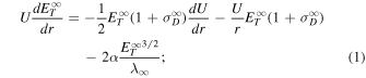

Equation (1) is derived by assuming zero 2D cross-helicity (i.e.,  , where 〈z∞±2〉 denotes the outward/inward 2D Elsässer energy) and Equation (2) by assuming
 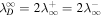 and
and  , where
  is the correlation length of the 2D residual energy
  − 〈B∞2〉/μ0
ρ), and
− 〈B∞2〉/μ0
ρ), and  is the correlation length of the 2D outward/inward Elsässer energy (see Zank et al. 2017, for the details). Here,
  ) is the normalized residual energy, U is the solar wind speed, and α and β are the von Kármán–Taylor constants. By dividing Equation (1) by
  and using Equation (2), we obtain
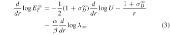
Integration of Equation (3) yields

where we assume  constant. Note that the normalized (2D/slab) residual energy may vary with radial distance (Adhikari et al. 2015, 2020, 2022a, 2022b; Zank et al. 2018a; Chen et al. 2020; Zank et al. 2021; Kleimann et al. 2023). The parameters
  , U0, and
  are the total 2D turbulence energy, solar wind speed, and the 2D correlation length at a reference point r0. Equation (4) is a solution of Equation (1), and it shows that
  is a function of solar wind speed, heliocentric distance, and the 2D correlation length. It is important to note that the presence of λ∞ controls the dissipation rate for
  , but it does not partition the turbulence energy into proton and electron heating rates. In the absence of the dissipation term, the solution takes the form

and it reduces to

for  . Equation (6) corresponds to a WKB-like solution of Equation (1) (bearing in mind that Equation (1) was not derived under the assumption of small-amplitude fluctuations, and linearity is imposed here post facto by neglecting the dissipation term), indicating that
  depends not only on r, but also on U. If
  , Equation (6) implies
  , similar to the result in Zank et al. (1996).
From Equations (2) and (4), we obtain

where  . Integration of Equation(7) yields
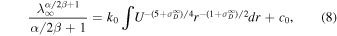
where c0 is the integration constant. To solve Equation (8), we assume a background profile for U of the form

where p denotes a scaling index for the solar wind speed and is obtained from observations. Equation (8) is then easily integrated for

where 
 and
and  . On using Equations (9) and (10), Equation (4) becomes
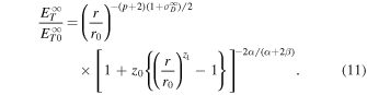
Equations (10) and (11) are the expressions for the 2D correlation length and 2D turbulence energy as a function of distance.
Using the relationship  + 〈B∞2〉/μ0
ρ = (rA
+ 1)〈B∞2〉/μ0
ρ =
+ 〈B∞2〉/μ0
ρ = (rA
+ 1)〈B∞2〉/μ0
ρ =  , where rA
is the Alfvén ratio, Equation (11) can be simplified as
, where rA
is the Alfvén ratio, Equation (11) can be simplified as
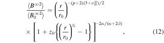
where  is the 2D fluctuating magnetic energy at r0. In the absence of the nonlinear dissipation term and
  , Equation (12) reduces to

which is a WKB-like solution. For a constant solar wind speed (i.e., p = 0), Equation (13) yields 〈B∞2〉 ∼ r−3, which is similar to the finding of Zank et al. (1996). Equations (12) and (13) are the expressions for the 2D fluctuating magnetic energy as a function of distance.
2.2. NI/slab Turbulence Transport Equations
The transport equation for the NI/slab total turbulent energy 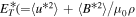 , where 〈u*2〉 is the slab turbulent kinetic energy, 〈B*2〉/μ0
ρ is the slab turbulent magnetic energy density, and 〈B*2〉 is the slab fluctuating magnetic energy) and the corresponding correlation length λ* can be expressed in the form (Zank et al. 2017; Adhikari et al. 2022b)
, where 〈u*2〉 is the slab turbulent kinetic energy, 〈B*2〉/μ0
ρ is the slab turbulent magnetic energy density, and 〈B*2〉 is the slab fluctuating magnetic energy) and the corresponding correlation length λ* can be expressed in the form (Zank et al. 2017; Adhikari et al. 2022b)

Equation (14) is derived by assuming equipartition between the slab fluctuating magnetic and kinetic energies. As before, Equation (15) is derived by assuming  and
and  , where
  is the correlation length for the slab outward/inward Elsässer energy and
  is the correlation length for the slab residual energy (see Zank et al. 2017, for the details). Here, VA
is the Alfvén velocity, and b(= 1/2) is the structural similarity parameter. We solve Equation (14) using Equation (15), and subsequently dividing by
is the correlation length for the slab residual energy (see Zank et al. 2017, for the details). Here, VA
is the Alfvén velocity, and b(= 1/2) is the structural similarity parameter. We solve Equation (14) using Equation (15), and subsequently dividing by  , to obtain

The magnetic field B, the solar wind mass density, and the Alfvén velocity are given by

where the radial profile for ρ is obtained from the conservation of mass, i.e.,  . B0, ρ0, and VA0 are the magnetic field, solar wind mass density, and the Alfvén velocity at r0. Using Equations (9) and (17), Equation (16) gives

where MA0 = U0/VA0 is the Alfvén Mach number. Integration of Equation (18) yields

where  and
and  are the slab turbulence energy and the slab correlation length at r0.
To find the solution for λ*, we integrate Equation (15), i.e.,

Using Equations (10), (11), and (17), Equation (20) gives

where 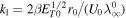 . Equation (21) can be numerically solved as

Equation (19) can then be written in the form

In the absence of the nonlinear dissipation term, Equation (23) reduces to the form

Similarly, the expression for the slab fluctuating magnetic energy 〈B*2〉 can be derived in the form

where  is the slab fluctuating magnetic energy at r0. Equation (25) reduces to

in the absence of the nonlinear dissipation term. We note that Equations (24) and (26) may not represent the WKB-like solutions, because the derivation of Equation (14) includes the mixing term (see Zank et al. 2017).
2.3. Proton and Electron Pressure Transport Equations
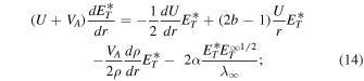
The transport equation for the electron pressure Pe is given by

where γe (= 5/3) is the polytropic index, νep is the collisional frequency between electrons and protons, Pp is the proton pressure, q e is the electron heat flux, and St e is the heating rate for electrons. Dividing the above equation by UPe and integrating with respect to r yields
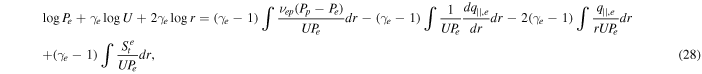
where we use ∇ · q e = 1/r2∂/∂r(r2 q∣∣,e ). To simplify the first integral on the right-hand side (rhs) of the above equation, we consider Pp − Pe ≈ Pp , assuming that the proton pressure is much larger than the electron pressure. Then, the first integral becomes (γe − 1)∫νep Pp /(UPe )dr. We also assume a linear relationship between νep Pp and UPe /r, qe and UPe , and St e and UPe /r, such that


where K0, Ke
, and Kq
are proportionality constants. Note that Equation (29) is similar to Equation (5) in Pine et al. 2020. However, their Equation (5) is related to proton heating, as shown in Equation (35) below. Although Equations (29) and (35) are presented in an approximate form derived through dimensional analysis to simplify the integration of their respective integrals, they describe the heating rates for electrons and protons, respectively. Unlike the partitioning of the turbulence energy into proton and electron heating rates, Equations (29) and (35) calculate the electron and proton heating rates, based on values of the parameters Kq
, Ke
, K0, and Kq
that yield analytical proton and electron temperatures similar to observations. There is a limitation in these equations, in that they are derived assuming a linear relationship. However, one can test the linear assumption using a 2D + slab dissipation rate =  , since the dissipation of turbulence energy is thought to be responsible for heating solar wind protons and electrons (Smith et al. 2006; Breech et al. 2009; Verdini et al. 2010; Usmanov et al. 2014; Zank et al. 2018b; Adhikari et al. 2021). In the right panel of Figure 7, we show the relationship between the 2D + slab dissipation rate and the proton + electron heating rate
  . Indeed, they show a linear relationship. Here, St
p
denotes the proton heating rate. In addition to their formulation being similar to Equation (5) in Pine et al. (2020), we verify their accuracy by comparing the solution for the proton + electron heating rate in these forms with the 2D + slab turbulent dissipation rate, as shown in the left panel of Figure 7. Similarly, Equation (30) describes the electron heat flux, and it is also similar to Equation (63) of Chandran et al. (2011). Equation (28) can then be solved easily for the electron temperature Te
as
. Indeed, they show a linear relationship. Here, St
p
denotes the proton heating rate. In addition to their formulation being similar to Equation (5) in Pine et al. (2020), we verify their accuracy by comparing the solution for the proton + electron heating rate in these forms with the 2D + slab turbulent dissipation rate, as shown in the left panel of Figure 7. Similarly, Equation (30) describes the electron heat flux, and it is also similar to Equation (63) of Chandran et al. (2011). Equation (28) can then be solved easily for the electron temperature Te
as

where Te 0 is the electron temperature at r0. We use Pe = ne kB Te , where ne is the electron density and kB is the Boltzmann constant. The 2D and slab turbulence may impact the parallel and perpendicular electron pressures (P∣∣ and P⊥, respectively) in different ways. However, here we only consider the scalar pressure, which includes the combined effect of 2D + slab turbulence.
Similarly, the transport equation for proton pressure Pp is given by
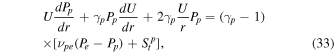
where γp (= 5/3) is the polytropic index and νpe is the collisional frequency between solar wind protons and electrons. Dividing the above equation by UPp and integrating with respect to r yields

To simplify the first integral on the rhs, as before, we suppose that the proton pressure is much larger than the electron pressure, so Pe − Pp ≈ − Pp . We then obtain −(γp − 1)∫νpe /Udr = − (γp − 1)K0∫Pe /(rPp )dr ≈ 0. Therefore, we neglect the first integral on the rhs of Equation (34). To integrate the second integral, we assume a linear relationship between St p and UPp /r, such that

where Kp is a proportionality constant. Equation (35) is similar to Equation (5) in Pine et al. (2020; see also Vasquez et al. 2007). Equation (34) can then be solved easily for the proton temperature Tp as

where Tp 0 is the proton temperature at r0. We use Pp = np kB Tp , where np is the proton density. As above, we only consider the scalar proton pressure. We also assume that the electron density is equal to the proton density (np ∼ ne ), to maintain charge neutrality. The values for the parameters Kp , Ke , and Kq can be obtained from the least-squares method, where we assume Ke = K0. Equation (36) with Kp = 1.24 yields the proton temperature with a radial profile of r−0.66, consistent with the result of Adhikari et al. (2022a).
We numerically solve the coupled transport equations describing the 2D and slab turbulence energies and correlation lengths (i.e., Equations (1), (2), (14), and (15)), and the proton and electron pressures (i.e., Equations (27) and (33)), using the background profiles described by Equations (9) and (17). In contrast to Equations (29) and (35), St p and St e can be obtained using a turbulent dissipation rate as (Smith et al. 2001; Verdini et al. 2010; Adhikari et al. 2015; Zank et al. 2018b; Adhikari et al. 2021)
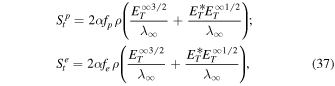
where fp and fe determine the fraction of turbulence energy for proton and electron heating rates, respectively. We note that, although Bandyopadhyay et al. (2023) and the left panel of Figure 4 show that the proton heating rate corresponds to about 80% of the total plasma heating rate near the Sun (∼13.3 R⊙), we use fp = 0.65 and fe = 0.33 because not all the turbulence energy is necessarily used to heat the solar wind protons and electrons (see the left panel of Figure 7, where the 2D + slab turbulent heating rate is slightly larger the proton + electron heating rate). We use the fixed values for fp and fe because the proton and electron heating rates change slightly in the range of distance 6.3–13.3 R⊙ (see the right panel of Figure 4). The collision frequency between proton and electron is given by (Zank et al. 2014a; Adhikari et al. 2023)

which is similar to Equation (13) of Cranmer et al. (2009). We use  . According to Cranmer et al. (2009), we can assume that νpe
∼ νep
. Similarly, we use the electron heat flux as (Bandyopadhyay et al. 2023)
. According to Cranmer et al. (2009), we can assume that νpe
∼ νep
. Similarly, we use the electron heat flux as (Bandyopadhyay et al. 2023)
where  and q0 = 0.01 erg cm−2 s−1.
3. Results
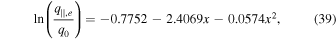
We calculate the background profiles for the solar wind speed, Alfvén velocity, and solar wind mass density using Equations (9) and (17). These equations are expressed as a function of radial distance, and they include a scaling index for the solar wind speed "p." We find p = 0.23 using a least-squares method for the solar wind speed values obtained from Telloni et al. (2023b; black dots in the left panel of Figure 1). This result implies that the solar wind speed increases as  between 6.3 R⊙ and 13.3 R⊙, as indicated by the black curve in the left panel of Figure 1, which overlays the black dots. Likewise, we plot the Alfvén velocity using Equation (17), indicated by a red curve in the left panel of Figure 1, showing that the Alfvén velocity decreases as
  , closely consistent with the Telloni et al. (2023b) results (red dots). Note that the red and black filled circles in the left panel are the PSP-measured Alfvén velocity and solar wind speed. Clearly, the Alfvén velocity is larger than the solar wind speed, as would be appropriate for a sub-Alfvénic flow. In the right panel of Figure 1, we plot the solar wind mass density (black curve), which shows that the solar wind mass density decreases as
  . The black curve is very similar to the result (black dots) of Telloni et al. (2023b), including the PSP-measured value (black filled circle). The radial profiles for the solar wind speed, Alfvén velocity, and solar wind mass density are incorporated in the analytical solutions for 2D and slab turbulence energies, as well as their corresponding correlation lengths, and the proton and electron temperatures. We also remind the reader that the Alfvén velocity is not included in the computation of the 2D turbulence energy and correlation length in the low βp
≪ 1 or βp
∼ 1 plasma beta regime.
. The black curve is very similar to the result (black dots) of Telloni et al. (2023b), including the PSP-measured value (black filled circle). The radial profiles for the solar wind speed, Alfvén velocity, and solar wind mass density are incorporated in the analytical solutions for 2D and slab turbulence energies, as well as their corresponding correlation lengths, and the proton and electron temperatures. We also remind the reader that the Alfvén velocity is not included in the computation of the 2D turbulence energy and correlation length in the low βp
≪ 1 or βp
∼ 1 plasma beta regime.
Figure 1. Left: Solar wind speed (black) and Alfvén velocity (red) as a function of distance. Right: Solar wind mass density as a function of distance. The black and red curves are obtained from Equations (9) and (17). The red and black dots are obtained from Telloni et al. (2023b), and the filled circles represent PSP-measured values.
Download figure:
Standard image High-resolution imageIn the left panel of Figure 2, we present the radial profiles for 2D and slab total turbulence energies with increasing distance. We use the following values for the parameters: α = 0.026, β = α/2,  , r0 = 6.3 R⊙, U0 = 264.06 km s−1, VA0 = 1.04 × 10³ km s−1, ρ0 = 8.57 × 10⁻¹⁸ kg m−3,
  km,
km,  km,
km,  km2 s−2, and
 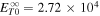 km2 s−2. In the left figure, the solid black curve identifies the slab turbulence energy, calculated from Equation (23), and the dashed cyan curve is the numerical solution. The two solutions are identical. The radial profile of
  follows an approximate
  profile, indicating an increase in slab turbulence energy with increasing distance in the sub-Alfvénic flow. The solid black curve closely aligns with the PSP-measured value (black filled circle) at 13.3 R⊙. The black dots and filled circles denote the outward-propagating Alfvén wave energy, and they are obtained from Telloni et al. (2023b). Note that the black dots are derived using the conservation of wave action approach (Velli 1993), which does not incorporate the dissipation of outwardly propagating Alfvén waves. Notably, the black dots exhibit a larger magnitude compared to the black curve, which includes the turbulent dissipation term. Here, the black dotted curve represents the analytical solution for slab turbulence energy in the absence of the dissipation term. Therefore, it does not include the loss of energy through turbulent dissipation, and it exhibits a more rapid increase, followed by a
  dependence, as compared to the solid black curve. We also note that this solution does not represent a WKB-like solution for slab turbulence energy, as Equation (14) also includes the mixing term (see Zank et al. 2017). The solid red curve and dashed green curve represent the analytical and numerical solutions for 2D turbulence energy
  , showing the same amplitude and a decrease characterized by an r−1.18 trend. Note that, at 6.3 R⊙, the value of
  is assumed to be four times that of
  . Similarly, the red dotted curve denotes the solution for
  in the absence of nonlinear dissipation term, which decreases as r−0.44, more slowly than the solution including the dissipation term.
Figure 2. Left: 2D (solid and dotted red and dashed green curves) and slab (solid and dotted black and dashed cyan curves) turbulence energies as a function of distance. The solid curves correspond to the analytical solutions that include the nonlinear dissipation term, and the dashed curves the numerical solutions. The dotted red and black curves are the analytical solutions without the nonlinear dissipation term. The blue dots are obtained from Telloni et al. (2023b), and the filled circle represents a PSP-measured value. Right: 2D (solid red and dashed green curves) and slab (solid black and dashed cyan curves) correlation lengths as a function of distance.
Download figure:
Standard image High-resolution imageIn the right panel of Figure 2, we show the radial profiles for the 2D and slab correlation lengths of the total turbulence energy as a function of heliocentric distance. The analytical and numerical solutions (solid red and dashed green curves) for the 2D correlation length are identical, and they increase with increasing distance. Similarly, the analytical and numerical correlation lengths for slab turbulence energy (black and dashed cyan curves) show the same magnitude and increase as a function of distance. Specifically, the 2D and slab correlation lengths follow radial profiles of r0.36 and r0.1, respectively.
In Figure 3 (left), we plot the radial evolution of the 2D 〈B∞2〉 and slab 〈B*2〉 fluctuating magnetic energies from 6.3 R⊙ to 13.3 R⊙. In the figure, the solid red and dashed green curves represent the analytical and numerical solutions for 2D fluctuating magnetic energy, while the solid black and dashed cyan curves represent the slab fluctuating magnetic energy. The dotted red and black curves denote the analytical solutions for 〈B∞2〉 and 〈B*2〉 in the absence of the nonlinear dissipation term. The 〈B∞2〉 follows a radial trend of r−3.41, while 〈B*2〉 has a radial profile of r−1.67. Conversely, the 2D and slab solutions in the absence of the nonlinear dissipation term exhibit radial profiles of r−2.68 and r−1.46, respectively. This indicates that the latter solution for 2D and slab fluctuating magnetic energy decreases more slowly than the previous solution. Additionally, both the 2D total turbulence energy and the 2D fluctuating magnetic energy decrease with increasing distance in the sub-Alfvénic flow. In contrast, the slab total turbulence energy increases, while the slab fluctuating magnetic energy decreases.
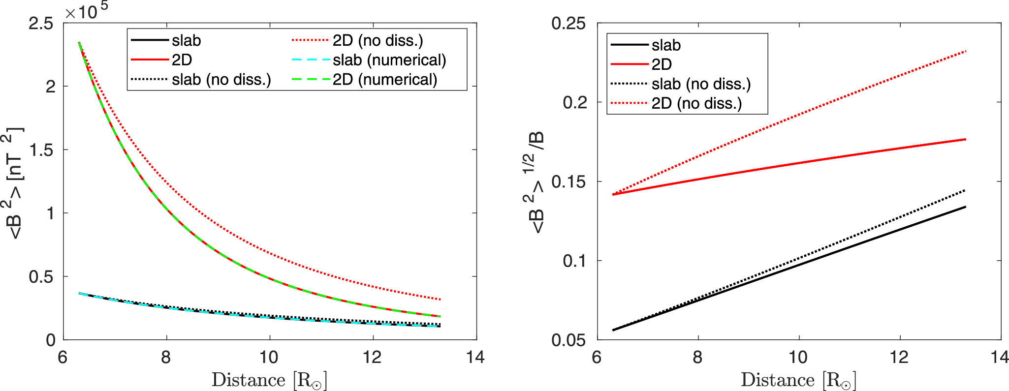
Figure 3. Left: 2D and slab fluctuating magnetic energies as a function of distance. Right: The ratio between the magnetic field fluctuations and the large-scale magnetic field as a function of distance. The solid black curve (and dashed cyan curve) and solid red curve (and dashed green curve) denote the analytical (and numerical) solutions that include the nonlinear dissipation term for the slab and 2D fluctuating magnetic energies, respectively. The dotted curves represent the solutions that neglect the dissipation term.
Download figure:
Standard image High-resolution imageIn Figure 3 (right), we show the ratio between 〈B∞2〉1/2 and B, as well as that of 〈B*2〉1/2 and B, as a function of distance. As the distance increases, the ratio of 〈B∞2〉1/2 and B (solid red curve) increases as r0.29, while the ratio of 〈B*2〉1/2 and B (solid black curve) increases as r1.17. Likewise, in the absence of the nonlinear dissipation term, 〈B∞2〉1/2/B and 〈B*2〉1/2/B increase as r0.66 and r1.27, respectively. This indicates that, in the latter case, the ratio increases more rapidly compared to the previous case.
In the left panel of Figure 4, we plot the temperatures of protons (solid black, solid green, and dotted black curves) and electrons (solid red, solid cyan, and dotted red curves) as a function of heliocentric distance. In the figure, the solid black and red curves denote the analytical results. The solid cyan and green curves represent the full numerical solutions. The dotted black and red curves correspond to the proton and electron temperatures obtained by Telloni et al. (2023b). To obtain the analytical results of the proton and electron temperatures, we use the following values: Kp = 1.24, Ke = 0.6, K0 = 0.6, and Kq = 0.6, Tp0 = 1.12 × 10⁶ K, and Te0 = 5.6 × 10⁵ K, where Tp0 and Te0 are the PSP-measured values at 13.3 R⊙. Note again that the Kp , Ke , and Kq values can be obtained from the least-squares method. These analytical results can exhibit different radial profiles for different Kp , Ke , and Ke values. Similarly, these values may change with heliocentric distance (Quataert 1998; Chandran et al. 2010; Howes 2010; Chen et al. 2020; Roy et al. 2022; Shankarappa et al. 2023). However, in the region of interest in this study, using fixed values for Kp , Ke , and Kq yields analytical results for the solar wind proton and electron temperatures, as well as the proton and electron heating rates, that are similar to the observed values measured by PSP. In addition, the analytical result for the proton temperature shows a radial profile of r−0.66, consistent with that of Adhikari et al. (2022a). The analytical result for the electron temperature is similar to the result of Telloni et al. (2023b), showing a radial profile of r−0.49. Similarly, in the left panel of Figure 6, the theoretical heat flux is close to the PSP-measured heat flux at ∼13.3 R⊙. Furthermore, the analytical results of the proton and electron temperatures are compared with their numerical results, where the numerical results decrease more rapidly than the analytical results. However, the analytical proton and electron temperatures are (1–1.04) and (1–1.13) times larger than their numerical solutions, indicating that they are relatively close. These comparisons gives us confidence that the analytical equations for proton and electron temperatures can be used to explain the observed proton and electron temperatures measured by PSP and SO, despite assuming Tp ≫ Te . The proton temperature (black curve) deviates from the result (black dots) of Telloni et al. (2023b). Note that Telloni et al. (2023b) traced back the proton temperature based on a radial profile of r−1 derived from the statistical analysis of proton temperatures in the super-Alfvénic solar wind flow.
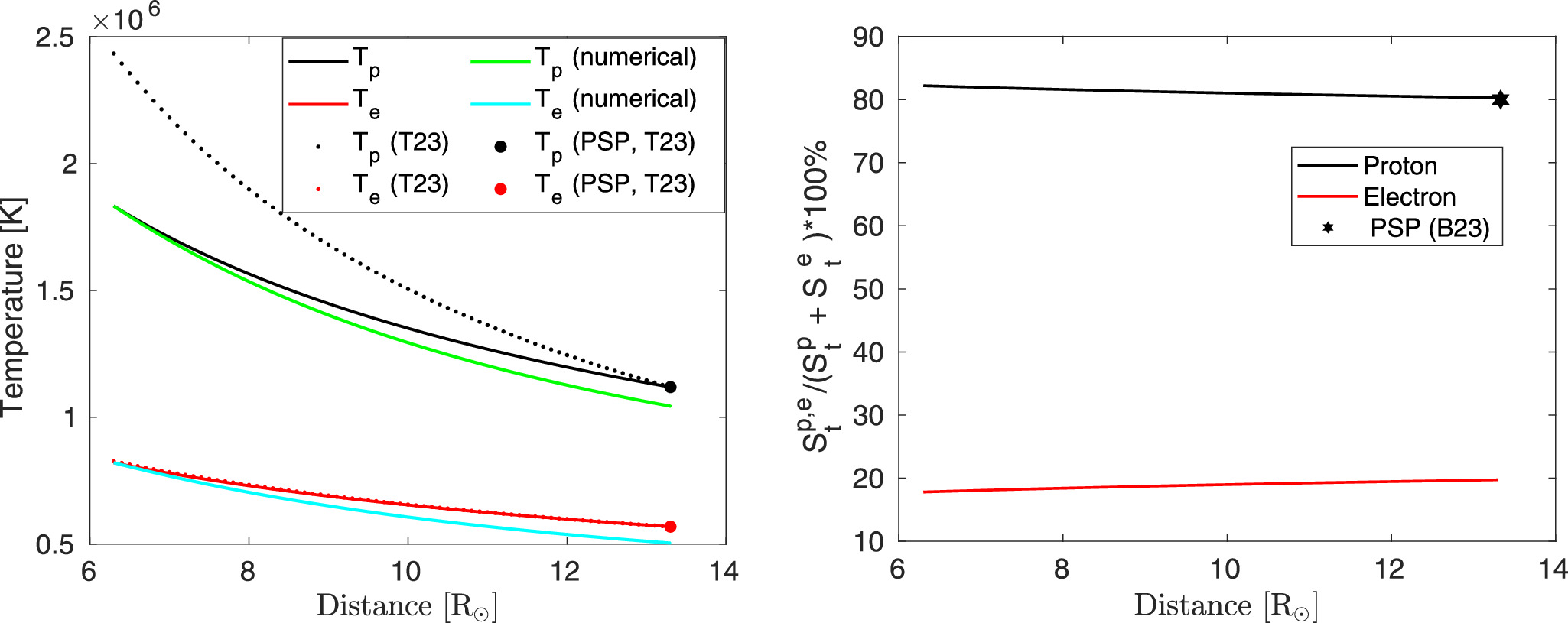
Figure 4. Left: Proton (black curve and circles) and electron (red curve and circles) temperatures as a function of radial distance. The red and black circles represent the results of Telloni et al. (2023b), and the solid red and black circles are the PSP-measured values. Right: Proton (black curve) and electron (red curve) heating rates as a function of radial distance. The black star is the result of Bandyopadhyay et al. (2023).
Download figure:
Standard image High-resolution imageThe right panel of Figure 4 plots the heating rate for protons (black curve) and electrons (red curve). These heating rates are calculated from Equations (35) and (29). At 6.3 R⊙, the proton heating rate accounts for approximately 82% of the total heating rate, exhibiting a slight decrease followed by an r−0.04 profile with increasing distance, and it is consistent with the result (black star) of Bandyopadhyay et al. (2023) at about 13.3 R⊙. Conversely, the electron heating rate at 6.3 R⊙ is about 18% of the total heating rate, and it increases with a radial trend of r0.14 as a function of distance.
Figure 5 shows the proton and electron temperatures (left panel) and their heating rates (right panel) for two cases: one in which the electron heat flux is neglected (Kp = 1.24, Ke = 0.9, K0 = 0.9, and Kq = 0), and the other in which both the electron heat flux and Coulomb collisions are neglected (Kp = 1.24, Ke = 1.5, K0 = 0, and Kq = 0). Note again that these values yield the radial profiles of the (analytical) proton and electrons temperatures as r−0.66 and r−0.45, respectively. In both cases, the proton and electron temperatures are identical. However, their heating rates differ. In the absence of electron heat flux, the electron heating rate ranges between 20% and 30% of the total heating rate (red dashed curve), larger than that (red curve) in the right panel of Figure 4. Consequently, this results in a decrease in the proton heating rate, ranging between 80% and 70% of the total heating rate (black dashed curve). In the absence of both the electron heat flux and Coulomb collisions, the electron heating rate further increases between 30% and 40% of the total heating rate, while the proton heating rate further decreases to the range of 70% and 60% of the total heating rate. In this case, the effects of 2D and slab turbulence on P∣∣ and P⊥ might be more relevant. However, we only consider the scalar pressure (or temperature) in this study.

Figure 5. The description of this figure is similar to that of Figure 4. Electron and proton temperatures and their heating rates are plotted in the absence of electron heat flux (Kp = 1.24, Ke = 0.9, K0 = 0.9, and Kq = 0), shown by dashed curves, and in the absence of both electron heat flux and Coulomb collisions (Kp = 1.24, Ke = 1.5, K0 = 0, and Kq = 0), shown by solid curves. In the left panel, the solid and dashed curves overlap with each other.
Download figure:
Standard image High-resolution imageThe left panel of Figure 6 shows the electron heat flux (black curve) as a function of distance. The electron heat flux decreases with distance according to  , and it is close to that (black star) of Bandyopadhyay et al. (2023), which was derived from PSP measurements. The right panel displays the collision frequency between electrons and protons (νes
) as a function of distance, exhibiting a radial profile of
, and it is close to that (black star) of Bandyopadhyay et al. (2023), which was derived from PSP measurements. The right panel displays the collision frequency between electrons and protons (νes
) as a function of distance, exhibiting a radial profile of  .
.
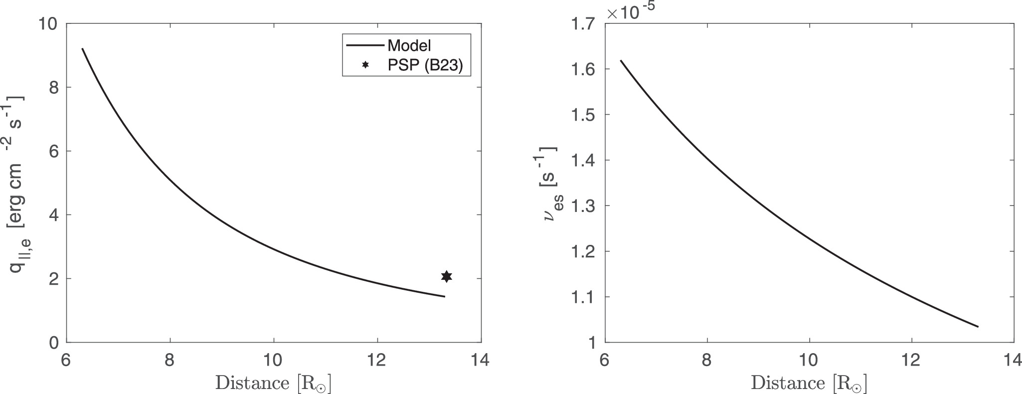
Figure 6. Left: Electron heat flux (Equation (30)) is plotted as a function of distance, and is compared with the result (black star) of Bandyopadhyay et al. (2023). Right: Collision frequency between electrons and protons (Equation (31)) is plotted as a function of distance.
Download figure:
Standard image High-resolution imageThe top left panel of Figure 7 shows the heating rates as a function of heliocentric distance. In the figure, the black curve denotes the turbulent heating rate, calculated from the dissipation terms for 2D and slab turbulence, i.e.,  (Equations (1) and (14)), where the first term inside the parenthesis corresponds to the dissipation of 2D turbulence and the second term to that of slab turbulence. The red curve denotes the proton + electron heating rate (
 ), calculated by adding the proton and electron heating rates, Equations (35) and (29). The heating rates are largest at 6.3 R⊙, and they decrease as a function of distance. The two heating rates are close, as shown in the bottom left panel, where their ratio ranges between 1 and 1.2. The 2D + slab turbulent heating rate is slightly larger than the proton + electron heating rate, where the previous heating rate decreases as r−3.77 and the latter heating rate as r−3.61. This may also indicate that all of the dissipated turbulent energy may not only heat the protons and electrons, but that some fraction of the dissipated turbulent energy may go into creating a nonthermal population of ions (e.g., stochastic acceleration by magnetic islands; Zank et al. 2014b; Khabarova & Zank 2017; Zhao et al. 2018; Adhikari et al. 2019), and a nonthermal population of electrons. The right panel of Figure 7 shows the relationship of the 2D+slab turbulent heating rate with the proton + electron heating rate. The solid curve lies above the dotted curve, which represents that the 2D + slab turbulent heating rate and the proton + electron heating rate are equal. It is evident that the previous heating rate exhibits a nearly linear relationship with the latter heating rate.
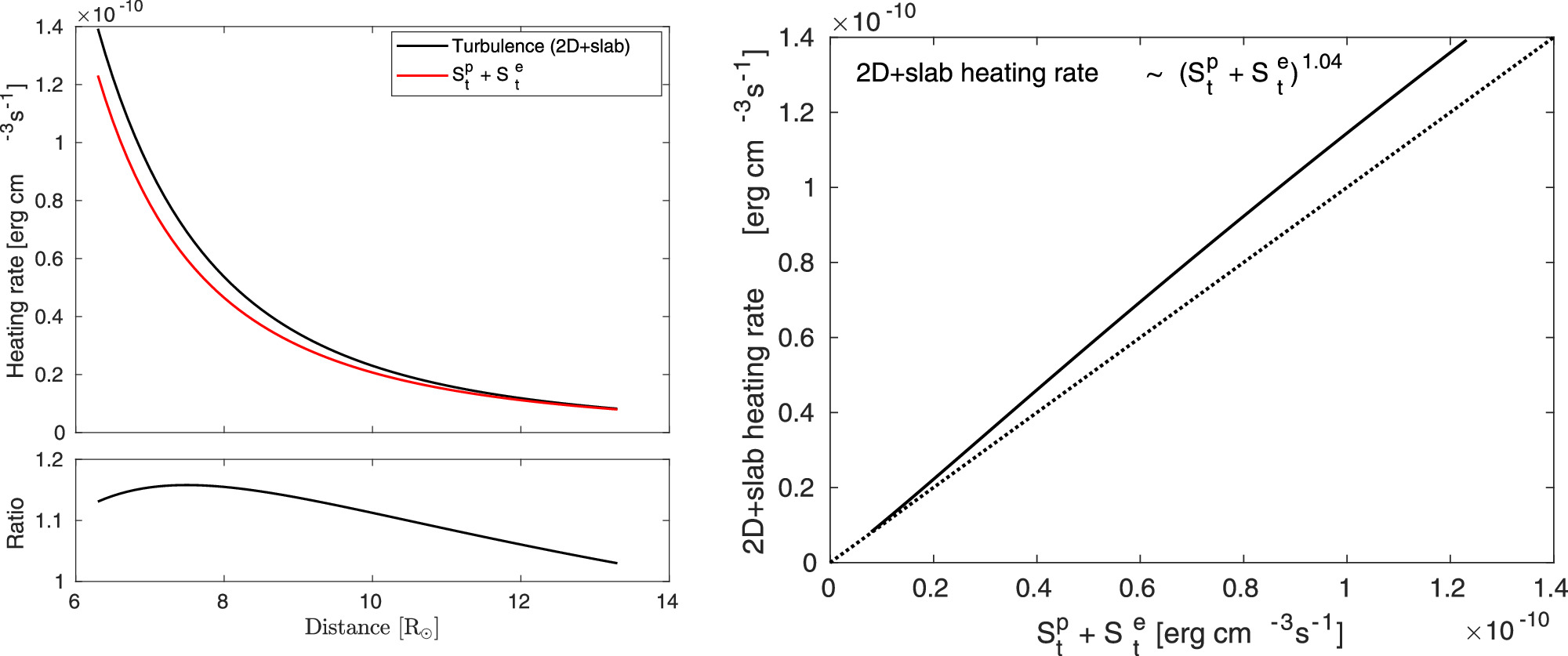
Figure 7. Top Left: Comparison of two heating rates as a function of heliocentric distance. The black curve is calculated using the dissipation term from 2D and slab turbulence. The red curve is calculated from  . Bottom Left: Ratio between two heating rates as a function of distance. Right: 2D + slab turbulent heating rate vs. proton + electron heating rate. The dotted line represents that the 2D + slab turbulent heating rate is equal to the proton + electron heating rate. See text for details.
Download figure:
Standard image High-resolution image4. Discussion and Conclusions
We presented analytical solutions for 2D and slab total turbulence and fluctuating magnetic energies, their correlation lengths, and the proton and electron temperatures for the sub-Alfvénic flow. These analytical solutions use background profiles for the solar wind speed, solar wind mass density, and Alfvén velocity. Specifically, our analytical solutions include a scaling index for the solar wind speed "p." We calculated the radial evolution of 2D and slab turbulence energies and correlation lengths, as well as the proton and electron temperatures and their heating rates in the extended solar coronal region between 6.3 and 13.3 R⊙. In addition, we also numerically solved the coupled transport equations describing the 2D and slab turbulence energies and correlation lengths, as well as the electron and proton pressures, and compared the analytical solutions with the PSP-measured values at about 13.3 R⊙, as well as the numerical solutions. We summarize our findings as follows.
- 1.The radial evolutions for the solar wind speed, solar wind mass density, and Alfvén velocity exhibit radial profiles of the form
 , , and , respectively. These radial profiles are closely aligned with the results of Telloni et al. (2023b), as well as PSP-measured values at 13.3 R⊙.
 - 2.The analytical solution for slab turbulence energy is consistent with the PSP-measured outward-propagating Alfvén wave energy at 13.3 R⊙ as reported by Telloni et al. (2023b), and it is consistent with the numerical solution of the slab turbulence energy. However, it is comparatively lower than the outward Alfvén wave energy obtained using the wave action conservation approach (Velli 1993), which neglects dissipation of the turbulence. The evolution of slab turbulence energy follows a radial trend of, and in the absence of the dissipative term, the slab turbulence energy exhibits a radial profile of .
- 3.The analytical solution for 2D total turbulence energy follows a radial profile of, while neglecting dissipation results in the analytical solution for the 2D total turbulence energy decreasing more slowly as . The analytical and numerical solutions for the 2D total turbulence energy are identical as a function of heliocentric distance.
- 4.The analytical and numerical solutions for 2D and slab correlation lengths follow radial profiles of the form and , respectively.
- 5.The analytical and numerical solutions for 2D and slab fluctuating magnetic energies exhibit radial profiles of and , respectively.
- 6.The ratio between the 2D magnetic field fluctuations and the large-scale magnetic field increases as, but more slowly than the ratio of the slab magnetic field fluctuations to the large-scale magnetic field .
- 7.The analytical solution for electron temperature follows a radial profile of, whereas the analytical solution for proton temperature follows . At 6.3 R⊙, the heating rate for protons accounts for about 82% of the total plasma heating rate, decreases according to , and becomes ∼80% of the total plasma heating rate at 13.3 R⊙, consistent with the result of Bandyopadhyay et al. (2023). Conversely, the heating rate for electrons at 6.3 R⊙ is about 18% of the total heating rate and increases as . If the electron heat flux is neglected, the proton heating rate falls between the range of 70% and 80% of the total plasma heating rate, while the electron heating rate increases and falls in the range between 30% and 20% of the total heating rate. If both the electron heat flux and Coulomb collisions are neglected, the heating rate for protons decreases further, ranging between 60% and 70% of the total plasma heating rate, while the electron heating rate increases further and ranges between 40% and 30% of the total plasma heating rate.
- 8.Although we assume that Tp ≫ Te , the analytical results for proton and electron temperatures are in fact relatively close to the numerical results for proton and electron temperatures, respectively.
- 9.The electron heat flux in the sub-Alfvénic flow has a radial profile of, and it is close to the estimate presented by Bandyopadhyay et al. (2023) at about 13.3 R⊙. The collision frequency between protons and electrons exhibits a radial profile of .


The analytical solutions presented in this manuscript provide valuable insight into turbulence in the sub-Alfvénic region of the solar corona, as well as coronal heating and solar wind acceleration. The analytical solutions provide a simple model against which to evaluate in situ and remote measurements made of the solar corona by PSP and SO, in particular with respect to modern turbulence theories thought to be responsible for the heating of the solar corona and acceleration of the solar wind.
Acknowledgments
We acknowledge the anonymous referee for providing helpful and constructive comments. We acknowledge the partial support of a Parker Solar Probe contract SV4-84017, an NSF EPSCoR RII-Track-1 cooperative agreement OIA-2148653, and NASA awards 80NSSC20K1783 and 80NSSC21K1319, as well as NASA Heliospheric Shield 80NSSC22M0164, and the SWAP instrument effort on the New Horizons project (M99023MJM; PU-A WD1006357), with support from NASA's New Frontiers Program and the IMAP mission as a part of NASA's Solar Terrestrial Probes (STP) mission line (80GSFC19C0027). This research was supported partially by the International Space Science Institute (ISSI) in Bern, through ISSI International Team project #560.
Appendix: NI/Slab Turbulence Transport Equations in the U ≫ VA Flow
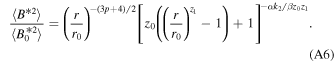
For U ≫ VA , Equation (16) can be simplified as

using b = 1/2. The integration of the above equation yields

Similarly, in a super-Alfvénic flow (assuming U ≫ VA ), Equation (15) reduces to

By substituting Equations (9), (10), and (11) into Equation (A3) and then integrating, we obtain

where 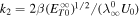 . We express Equation (A2) in terms of distance as
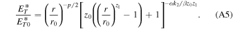
Equation (A5) shows that the slab turbulence energy decreases with increasing distance in the super-Alfvénic (U ≫ VA ) flow. Similarly, the slab fluctuating magnetic energy can be expressed in terms of radial distance as
Equations (A4), (A5), and (A6) show the radial dependence of the correlation length, total turbulence energy, and the fluctuating magnetic energy of slab turbulence in the super-Alfvénic solar wind flow.